| Issue |
BIO Web Conf.
Volume 17, 2020
International Scientific-Practical Conference “Agriculture and Food Security: Technology, Innovation, Markets, Human Resources” (FIES 2019)
|
|
|---|---|---|
| Article Number | 00218 | |
| Number of page(s) | 5 | |
| DOI | https://doi.org/10.1051/bioconf/20201700218 | |
| Published online | 28 February 2020 | |
Simulation of drip irrigation on slope lands
1
Cheboksary Cooperative Institute, Cheboksary 428025, Russia
2
Chuvash State University, Cheboksary 428015, Russia
* Corresponding author: serg.chuchkaloff@yandex.ru
One of the main tasks of drip irrigation is to predict the geometric parameters of the moisture contours by estimating the impact of the water rate and the irrigation water on the moisture distribution in the soil. In this paper the soil water retention curve and function of moisture conductivity are used to simulate the process of moisture movement taking into account both the state and the type of soil. A software tool has been developed to automate calculations and visualize them. One of the main advantages of this software tool is that it allows using three-dimensional arrays of porosity values, specific surface area and initial soil moisture for each elementary volume of soil. The results of simulating various initial conditions make it possible to form contours and maintain optimum soil moisture right in the area of the plant root zone development. The correspondence of the simulation results to real data was verified by a series of laboratory and field experiments having light-gray forest soil. The calculated coefficients of determination have average values, that are quite high for such tasks, namely 0.68 (horizontal surfaces) and 0.72 (inclined surfaces).
© The Authors, published by EDP Sciences, 2020
 This is an Open Access article distributed under the terms of the Creative Commons Attribution License 4.0, which permits unrestricted use, distribution, and reproduction in any medium, provided the original work is properly cited.
1 Introduction
Drip irrigation [1], which is widespread in the countries suffering from fresh water shortage and having large proportion of arid areas, is gradually winning application in Russia. Continuously increasing demand for fresh water encourages agricultural producers to switch to this irrigation method for economic reasons [2].
When applying drip irrigation, one of the important tasks is to determine the geometric parameters of the resulting moisture contours in the area of root zone development. Information about the depth, width and shape of the moisture contour allows providing the root system with water, fertilizers etc., ideally without any extra costs.
Contour shape and size may vary considerably and depend essentially on the rate, quantity and quality of feed water, the presence of dissolved fertilizers, and the water-physical properties as well as on the soil condition. Since the contour shape and size are closely related to irrigation rates, the calculation of their dynamics is necessary to optimize and improve the economic efficiency of drip irrigation. The distribution of moisture in drip irrigation has its own characteristics, which in most recent studies [3, 4] are expressed in the form of regression dependencies that approximately describe the dynamics of geometric shapes of contours for different moisture values.
The study of the moisture contours parameters for different irrigation rates is often carried out on water-balance areas and at the initia stage it is of a descriptive statistical character. In some cases, the dependence of the supplied water volume on the number of emitters and their location relative to the plants is studied, and a method for calculating a water volume for a single emitter is used then re-count is made per 1 ha. In this regard the following factors are taken into account [5, 6]: the degree of initial soil moistening of a plot, soil type, climate, permeability, porosity, salinity, compaction of the soil profile etc. Installing moisture sensors at different depths or taking samples with the help of drills allows obtaining and analyzing moisture values. Then, in most cases, regression equations expressing the dependence of the shapes and sizes of the moisture contours on the above factors are obtained by processing an array of statistical data.
This approach is not always applicable to the extrapolation of the findings for the same soils are in a more compacted and loosened state, not to mention other types of soils. However, despite some unsolved problems, in particular, the problem of the influence of drip irrigation on the physical and chemical properties of the soil [7], drip irrigation allows maintaining the optimal water regime of soils in the most cost-effective and environmentally friendly way.
Since the calculation of drip irrigation regimes allows dosing the water supply directly to the location of the crop root zone, it is logical to use the soil water retention curve (SWRC) and the moisture conductivity function as the basis for numerical calculations in simulating. SWRC determines the dependence of the soil moisture pressure on the moisture content. The moisture conductivity function binds the SWRC and the moisture conductivity coefficient that in its turn also depends on the moisture content. SWRC and moisture conductivity function are directly dependent on the physical and mechanical properties of soils. They allow full and clear determining the moisture movement in the soil.
At present there is a large number of functions models [8, 9] of soil water retention and moisture conductivity capacity (e.g., such as HYDRUS [10]), but as a rule because of a large array of input constants and statistical calculations validity from physical point of view is hardly to be seen. Soils of the Chuvash Republic (Russia) have poor natural fertility and need external control of soils water regime. Therefore, to select the optimal irrigation regimes and rates that could provide the formation of proper moisture contours the hydro-physical approach seems to be more preferable in comparison a statistic descriptive one.
2 Materials and methods
Considering soil moisture as a phase having a contact surfaces with soil air and with the solid phase of the soil, let us make the analysis of the interaction of the components of the air-water-soil system within the energy approach [11]. The moisture movement in the soil is determined by the soil moisture potential gradient ψ=E/m (energy to water mass ratio) or by equivalent pressure p=ρψ (where ρ is water density). The value of the potential is made up of the interaction of moisture with the solid soil phase ψ′ and soil air ψ″. Thus, the function of moisture conductivity of soil and SWRC are determined. In the study [12] the following expressions are obtained for the soil moisture potential gradient ψ and the hydraulic conductivity (moisture conductivity) K(w):
![$$ \begin{gathered} \psi = \psi ^{\prime} + \psi ^{\prime\prime} = \frac{{A\Omega _{0}^{3} }}{\rho }\left[ {\frac{1}{{w^{3} }} - \frac{1}{{\Pi _{0}^{3} }}} \right] + \hfill \\ + \frac{{\Omega _{0} \sigma _{{\lg }} }}{\rho }\left( {1 - \frac{w}{{1 - \Pi _{0} + w}}} \right) \cdot \left( {1 - \frac{w}{{\Pi _{0} }}} \right)^{{2.5}} , \hfill \\ \end{gathered} $$](/articles/bioconf/full_html/2020/01/bioconf_fies2020_00218/bioconf_fies2020_00218-eq1.gif)
![$$ K(w) = \frac{{\pi ^{2} }}{{\Omega _{0} \eta S_{2} }} \cdot \frac{{\lambda \Pi _{0}^{{2.5}} }}{{1 - \Pi _{0} }} \cdot \left[ {1 - \left( {1 - \frac{w}{{\Pi _{0} }}} \right)^{2} } \right], $$](/articles/bioconf/full_html/2020/01/bioconf_fies2020_00218/bioconf_fies2020_00218-eq2.gif)
where Ω0 – volumetric specific surface (m2/m3), w – volumetric water content (m3/m3), σlg – specific free surface energy at the water/air boundary (J/m2), ρ – water density (kg/m3), A – the dimensional constant (J), Π0 – the porosity of the dry soil sample (m3/m3), η – water viscosity (Pa∙s), S – cross-section area of soil sample the water flows through (m2), and λ – dimensionless coefficient.
During the experimental studies with light-gray forest soil in the laboratory and in the fields, it was found that the solid soil phase is neither deformed nor washed off, the water temperature in the soil and the temperature of irrigation water are equal, the salt concentration is low, and the absorption of water by the plant roots and evaporation are negligible. These facts allowed simplifying the computational model within a number of approximations.
The use of formulas (1) and (2), at the present level of computing power, allows abandoning the use of Richards differential equations of moisture conductivity and use the Darcy difference equations. The problem of determining the contours of moisture in drip irrigation is generally three-dimensional. It can be reduced only with a zero slope of the irrigated surface to a two-dimensional problem with cylindrical symmetry with an emitter located on the axis.
The calculation of the moisture contours is carried out by setting the volume of moisture entering the point (cube with edges of ∆h=1 mm) of the upper layer per unit of time. In the process of calculating the potential difference of soil moisture, the gravitational potential g∆h is added when calculating the moisture transfer between adjacent horizontal soil layers and is not added when calculating the moisture transfer inside the horizontal soil layers.
Vertical and horizontal moisture transfer is calculated simultaneously by solving two Darcy equations and assuming that the moisture pressure in the soil volume receiving water is not higher (modulo) than the pressure in the soil volume losing water.
The Darcy formulae are used to calculate the amounts of moisture that flew out of the cylindrical element into the element located more far from the axis (∆Vhor, horizontal) and into the bottom element (∆Vver, vertical) respectively:
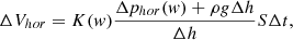
where K(w) – coefficient of moisture conductivity, ∆phor – pressure difference of soil moisture in the adjacent horizontal elements of the soil (Pa), ∆pver – pressure difference of soil moisture in the adjacent vertically arranged elements of the soil (Pa), S – the area of the element basis (m2), and ∆t – time (s).
3 Results and discussion
The software package written in the language of visual programming Delphi 10 was made and used to automate calculations. The visualization of calculations was performed using Golden Software Surfer 15.
The experiments were carried out on light-gray forest soil with zero slope and a slope of i=11°. A specific surface of soil particles Ω0 was 46.2 m2/g and porosity П was 0.53. In the calculations, the moisture increase with depth increase was simulated by the values of the initial moisture distributions, linearly increasing with depth increase from w=0.39 to w=0.42. The volume of the supplied water varied from 0 to 0.5 l and from 0 to 2 l. The agreement of the results of the experiment and simulation are given in table 1 with determination coefficients for different values of dripping water volume.
The visualization of calculations for drip irrigation is presented in Fig. 1 (without slope) and Fig. 2 (with slope). As shown in Fig. 1 and 2, the presence of slope has almost no effect on the initial stage of irrigation, and the left columns of the figures do not differ from each other. However, the right columns differ and illustrate a drain formation when there is a slope. Thus, the simulation demonstrates that the slope irrigation regimes chosen are incorrect that was proved by the experiments.
A particular feature of the developed software is that it makes the use arrays of such values as porosity, specific surface area and initial moisture for each elementary volume of soil, that are applied to calculate the coefficients of moisture conductivity and soil moisture pressure possible. Automatic mode allows calculating the moisture distribution during sprinkler and drip irrigation, which is necessary when specifying certain geometric parameters of moisture contours as well as in calculating the irrigation rates and periods that depend on hydro-physical soil properties.
Determination coefficients
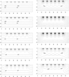 |
Fig. 1. Dynamics of the soil moisture contours in time with drip irrigation: zero slope (linear dimensions in cm are indicated on the vertical and horizontal axes). |
 |
Fig. 2. The dynamics of the soil moisture contours in time with drip irrigation: slope 11° (linear dimensions in cm are indicated on the vertical and horizontal axes). |
4 Conclusion
The software tool has been theoretically justified and developed for calculating the soil moisture contours. It allowed establishing the regularities of soil moisture contours formation when different amounts of water are supplied regardless of the initial soil moisture, as well as to trace the dynamics of contours parameters modification during irrigation. As an example we have given the calculation of the moisture contours of light-gray forest soils during drip irrigation. It was found that for a certain period of time from the moment of the
beginning of irrigation, the influence of the slope does not appear. Afterwards the shape of the contours undergoes distortion due to the slope and the drain is formed. The study of the dynamics of the contours of soil moisture during drip irrigation allows optimizing the norms and periodicity of irrigation.
At this stage we do not consider the impact of salts on increasing the potential of soil moisture in our calculations. We are planning to use the Van Goff formula and to correct the formula for SWRC for this purpose. We are also planning to include the value of the suction pressure of a particular plant into the SWRC formula to calculate water absorption by the roots of the plants. The temperature differences between soil and irrigation water should be taken into account according to the heat balance formulae that allows correcting the values of viscosity and surface tension coefficients.
Acknowledgments
The work was supported by RFBR, project No. 18-416210001 p_a.
References
- M. Albaji, M. Golabi, S. Boroomand Nasab, F.N. Zadeh, J. Saudi, Soc. Agric. Sci., 14(1), 1 (2015) [Google Scholar]
- N. Devika, A. Narayanamoorthy, P. Jothi, J. Rural Dev., 36(3), 293 (2017) [Google Scholar]
- K. Ramah, P. Santhi, G. Thiyagarajan, Madras Agric. J., 98 (1-3), 51 (2011) [Google Scholar]
- J. Reyes-Cabrera, L. Zotarelli, M.D. Dukes, D.L. Rowland, S.A. Sargent, Agr. Water Manage, 169, 183 (2016) [CrossRef] [Google Scholar]
- T. Selim, R. Berndtsson, M. Persson, Irrig. Drain., 62(3), 352 (2013) [Google Scholar]
- W. Fan, G. Li, IOP Conf. Ser. Earth Environ. Sci., 121, 052402 (2018) [Google Scholar]
- M. Mursec, J. Leveque, R. Chaussod, P. Curmi, Plant Soil Environ., 64, 20 (2018) [CrossRef] [Google Scholar]
- V. Too, C. Omuto, E. Biamah, J. Obiero, OJMH, 4, 173 (2014) [CrossRef] [Google Scholar]
- K.S. Perkins, Hydraulic Conductivity Issues, Determination and Applications, 419–434 (IntechOpen, London, 2011) [Google Scholar]
- M. Rowshon, H. Muhammed, M. Mojid, A. Ruediger, M. Soom, Pertanika J. Sci. & Technol., 27(1), 205 (2019) [Google Scholar]
- I. Maksimov, V. Alekseev, S. Chuchkalov, IOP Conf. Ser.: Earth Environ. Sci., 226, 012067 (2019) [CrossRef] [Google Scholar]
- V.V. Alekseev, I.I. Maksimov, Eurasian Soil Sci., 46(7), 751 (2013) [CrossRef] [Google Scholar]
All Tables
All Figures
|
Fig. 1. Dynamics of the soil moisture contours in time with drip irrigation: zero slope (linear dimensions in cm are indicated on the vertical and horizontal axes). |
| In the text | |
|
Fig. 2. The dynamics of the soil moisture contours in time with drip irrigation: slope 11° (linear dimensions in cm are indicated on the vertical and horizontal axes). |
| In the text | |
Current usage metrics show cumulative count of Article Views (full-text article views including HTML views, PDF and ePub downloads, according to the available data) and Abstracts Views on Vision4Press platform.
Data correspond to usage on the plateform after 2015. The current usage metrics is available 48-96 hours after online publication and is updated daily on week days.
Initial download of the metrics may take a while.