| Issue |
BIO Web Conf.
Volume 17, 2020
International Scientific-Practical Conference “Agriculture and Food Security: Technology, Innovation, Markets, Human Resources” (FIES 2019)
|
|
|---|---|---|
| Article Number | 00114 | |
| Number of page(s) | 7 | |
| DOI | https://doi.org/10.1051/bioconf/20201700114 | |
| Published online | 28 February 2020 | |
Migration of safety indicators for milk produced in the Oryol region
1
Oryol State University named after I.S. Turgenev, 302026 Oryol, Russia
2
K.G. Razumovsky Moscow State University of Technologies and Management (the First Cossack University), 109004 Moscow, Russia
3
Oryol State Agrarian University named after N.V. Parakhin, 302019 Oryol, Russia
* Corresponding author: This email address is being protected from spambots. You need JavaScript enabled to view it.
Abstract
The paper reports the milk safety indicators resulting from monitoring activities to predict and estimate high-quality milk materials in the Oryol region. The results of the study allow for predicting milk safety indicators for different milking periods. The study shows that milk produced in July, August, and September is the most suitable for production of functional dairy products, since such milk contains no aflatoxins and a minimum amount of toxic elements in this period.
© The Authors, published by EDP Sciences, 2020
 This is an Open Access article distributed under the terms of the Creative Commons Attribution License 4.0, which permits unrestricted use, distribution, and reproduction in any medium, provided the original work is properly cited.
1 Introduction
Safety indicators for produced milk primarily rely on certain natural factors, in particular the quality of forage. Milk xenobiotics are known to enter the human body through the soil – plant – animal – milk – people food chain.
Today, it is relevant to improve the quality of milk and obtain functional dairy products. Therefore, it seems to be very interesting to study the migration of toxic substances in produced milk, depending on definite regions and different milking periods, since the quality of forage in spring, summer, autumn-winter, and winter seasons varies significantly [1].
2 Results and discussion
The level of radioactive contamination in the Oryol region as a whole and for certain areas of the region is determined, and radioactive background is constantly monitored.
Toxic elements, aflatoxin M1, radionuclides are constantly monitored in the produced milk in line with SanPiN 2.3.2.1078-01 [2].
There are numerous data that highlight likely causes of certain toxic accumulations by plants and the ways, particularly via food chains, toxic substances are transferred to the human body. It is increasingly interesting to analyze the monitoring results towards toxic substances in produced milk subject to a season [3].
The number of sampled dairy products exposed to safety analysis at the Center for State Sanitary and Epidemiological Supervision in the Oryol Oblast is on average 1300–1500 per year, of which the milk produced accounts for about 50 %. Therefore, 500 milk samples were used for statistical estimation. Three levels of contamination were distinguished as per the content of toxic substances:
minimum level 1 – 33 % of the standard value;
medium level 2 – 33–66 % of the standard value;
maximum level 3 – 66–100 % of the standard value.
Toxic elements, aflatoxin M1 and radionuclides were estimated in the produced milk. The contamination levels are given in Table 1.
A statistical study based on a PC software package involved measuring the content of toxic, radioactive substances and aflatoxin M1 in the produced milk at different periods of the year. To successfully address these challenges, it is necessary to:
have enough data for statistical estimates (for annual observations – at least five levels, for seasonal – a least three seasonality periods);
ensure methodological comparability of data;
based on a thoroughly evaluated indicator, substantiate the possibility of transferring recent past patterns to the selected prediction period;
get an adequate mathematical model for further point and interval estimations.
The main form of statistical representation is observed time series (TS). The purpose of time series analysis is to study the relationship between regular and random behavior in the values of the levels of a series and to estimate a quantitative impact [4, 5].
Statistical methods present the levels of a series as a sum of several components, reflecting the regularity and randomness of development, in particular, as a sum of several components: (1)
(1)
where f(t) is a trend that, being a deterministic component, represents a steady change in the indicator over a long period of time and expresses the analytical function to form forecast estimates; S(t) is a seasonal component characterizing stable intra-annual fluctuations in the levels. It is represented by quarterly and monthly data (the presence of stable fluctuations in daily or weekly data can be considered as a cyclical phenomenon and thereof displayed by a seasonal component); E(t) is a residual component that represents the discrepancy between the actual and measured values (provided that an adequate (good) model is developed, then E(t) is close to 0, random, independent, attributable to standard component distribution, otherwise the model is considered bad).
The levels of a series are formed against the laws of three main types: inertia of a trend, inertia of the relationship between the studied indicator and indicators-factors that have a causal effect on it. Hence, there are specific problems for trend analysis and modeling, the relationship between the studied indicator and indicators-factors. The first problem is addressed through component analysis, the second through adaptive methods and models, and the third – through econometric modeling based on correlation-regression analysis.
The algorithm for statistical component analysis is associated with the following procedures: problem statement and source information selection; pre-analysis of source time series and formation of a set of prediction models; numerical estimate of model parameters; model quality assessment (adequacy and accuracy); selection of one best or development of a generalized model; point and interval predictions.
The problem statement was designed based on a meaningful analysis of the process; decision making on the choice of an indicator to characterize to the greatest extent; selection of indicators to influence the course of development; selection of the most reasonable prediction period, the optimal forecast horizon determined individually for each indicator, taking into account its stability and statistical data variability (usually it does not exceed 1/3 of a data set).
The pre-analysis involved matching the data available to the conditions required, via mathematical methods (objectivity, comparability, completeness, uniformity and stability). A flow chart was provided to measure the dynamics including gains, growth rate, increment rate, and autocorrelation coefficients.
A set of models (a source base of models) is formed on the basis of intuitive techniques, such as flow chart analysis of a series, formalized statistical procedures (evaluation of level gains). As such, it is desirable to use the simplest, most meaningful PC-based models with measurements to be supported by all models and methods available [6].
Thus, a model (graph and function equations) was based on:
data on toxic elements, aflatoxin M1 and radionuclides;
the number of milk samples with a maximum, medium and minimum level of contamination by toxic elements, aflatoxin M1 and radionuclides in the first, second, third and fourth quarters;
permitted levels and average content of toxic elements, aflatoxin M1 and radionuclides in samples recorded in individual quarters.
All necessary data are given in Tables 2–10.
By way of an EXCEL package, a functional relationship was as follows: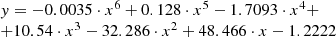 (2)
(2)
However, this kind of polynomial caused certain difficulties for a flow chart design (description and forecasting are rather difficult due to a large number of changing variables). Therefore, the next step was the problem statement to determine every single function for each graph separately.
Upon the points specified, it was necessary to obtain functional relationships through the method of least squares.
The least-squares method is a standard approach for the numerical estimation of parametric curves. The quality of a model is estimated against the minimum root-mean-square error. Observations approximated by complex functions provide a good fit to the actual data, but reduce the stability of the model during the forecasting period.
Extrapolation of a model curve over the observation period t = N+1, N+2 ... is the basis for predicting trend models. The interval estimation at each forecast point is determined by regression relationships with a user-defined confidence coefficient.
For x-value and y-value, the “best” is the linear function y = a + bx (for a given set of observed data), since it is optimal for all curves [5, 6].
The functional relationships resulting from all necessary calculations and data processing for all curves are based on the predicted trend series.
Linear trend estimation is used to monitor the changes in the trend of the object, analyze and predict the “behavior” of the object.
It is necessary to constantly monitor the dynamics of trend lines.
Contamination levels of the produced milk are given in Tables 2–13.
Based on the results, the number of milk samples with a minimum contamination by copper amounted to 22.00–54.20 %, the number of samples with a medium contamination amounted to 34.00–51.40 % and that with a maximum contamination – 11.80–30.20 %. Thus, the largest number of samples with a minimum copper contamination occurred in the third quarter.
The largest number of samples with a maximum contamination (150 and 120) was recorded in the first and second quarters. This can be due to the fact that copper is a fairly mobile element that forms stable complex compounds involving various functional groups. It is easily transferred from the soil to leaves [7] and normally reaches its maximum value in the second vegetation stage – May, June (the second quarter).
In a later period (July, August, September), copper mostly migrates to the root system or is washed off from the surface of plants with moisture. The highest average copper content was also recorded in the second quarter.
A functional relationship based on the predicted trend lines for copper is y=22,5.This means that for four quarters the value of copper along the trend line remains unchanged. The fitted curve for copper is shown in Fig. 1.
According to the results, the number of milk samples with a minimum contamination by zinc amounted to 27.80–60.60 %, the number of samples with a medium contamination amounted to 35.20–54.40 % and that with a maximum contamination – 4.20–23.40 %.
The number of samples with a maximum zinc level significantly differs, namely: 16.60–23.40 % in the first, second and fourth quarters, and only 4.20 % in the third quarter. This is due to the fact that zinc intensively enters plants at the beginning of vegetation and growth stages. It accumulates in leaves, generative organs and growing points [8].
The permitted zinc content is 5.0 mg/kg, a monitoring analysis showed the lowest zinc content in the milk in the third quarter, 38 % of the permitted level. The data distinguish the third quarter both in the number of samples with a minimum contamination, and in the average content of zinc in the milk.
A functional relationship based on the predicted trend lines for zinc is y = −1,7 · x + 28. The fitted curve is shown in Fig. 2.
The monitoring feedback showed the number of milk samples with a minimum contamination by lead amounting to 21.80–42.20 %, the number of samples with a medium contamination amounting to 43.20–57.80 % and that with a maximum contamination – 14.60–20.40 %. Thus, the number of samples with different levels of lead contamination in individual quarters just slightly varied.
However, the highest percentage of samples (42.20) with a minimum level of lead was recorded in the third quarter. This can be due to the fact that during the spring, when lead accumulates in the upper parts of plants, the number of samples with a minimum level is insignificant (in the second quarter – 29.80 %).
The way lead commonly enters plants from the environment is that hairy or waxy cuticles of leaves and fruits fix it. Some portion of lead is absorbed by the cell walls of leaves. Lead accumulates in the form of pyro- and orthophosphates, bound to soluble small molecules of proteins, and some carbohydrates. The absorption of lead by plants increases at a pH close to acidic [9]. When absorbed by the upper parts of plants, lead cannot be quickly transferred to the roots. It is usually transferred to the roots by the end of summer.
The permitted level of lead is 0.1 mg/kg. The lowest lead content in milk recorded in the third quarter made up 0.9 % of the standard level.
A functional relationship based on the predicted trend lines for lead is y = −1,1 · x + 29. The fitted curve is shown in Fig. 3.
As evidenced, the number of milk samples with a minimum contamination by cadmium amounted to 26.60–41.20 %, the number of samples with a medium contamination amounted to 55.00–65.40 % and that with a maximum contamination – 3.80–8.80 %.
The highest percentage of samples (41.20) with a minimum cadmium content was recorded in the third quarter. This can be owing to the fact that cadmium is a fairly mobile element that easily moves from the soil to the leaves. Once in plants, it is easily transferred in the form of organometallic compounds. Cadmium ions form mobile protein complexes. They are concentrated in the protein fraction of plants. They also interact with sulfhydryl and phosphate groups of some compounds. Cadmium gets easily involved in metabolic reactions with active substances located on the cell walls [10].
Cadmium accumulates in mature plants most intensively during the haymaking period. In the autumn-winter period, animals mainly live on hay and that explains the fact that cadmium reaches its maximum value in the first and fourth quarters.
The permitted level of cadmium is 0.005 mg/kg. The lowest cadmium content in milk recorded in the third quarter constituted 0.67 % of the standard level (in the first, second and fourth quarter it constituted 16.67 % of the standard level).
Milk produced in the third quarter had the lowest cadmium content.
A functional relationship based on the predicted trend lines for cadmium is y = −0,2 · x + 31 .The fitted curve is shown in Fig. 4.
The number of milk samples with a minimum contamination by mercury amounted to 38.20–45.80 %, the number of samples with a medium contamination amounted to 48.60–54.60 % and that with a maximum contamination – 4.20–8.80 %.
For four quarters, the average mercury in milk is 2.00–4.00 % of the standard level.
Mercury mainly accumulates in the vegetative organs of plants [11].
A functional relationship based on the predicted trend lines for mercury is y = −1,1 · x + 28,5. The fitted curve is shown in Fig. 5.
The number of milk samples with a minimum contamination by arsenic amounted to 26.20–52.40 %, the number of samples with a medium contamination amounted to 35.60–54.70 % and that with a maximum contamination – 10.60–22.20 %.
The permitted level of arsenic is 0.05 mg/kg. The average value of arsenic for four quarters remained unchanged and amounted to 40.00 % of the standard level.
Arsenic entry into plants depends not only on its concentration in the soil, but also on the type of plants and the texture of the soil. The use of phosphate fertilizers increases the natural level of arsenic in the soil [12].
The largest percentage of the total number of samples (22.20) with the highest level of arsenic contamination was recorded in the fourth quarter. This can be due to the fact that arsenic accumulates intensively when stored in root crops and hay.
A functional relationship based on the predicted trend lines for arsenic is y=−3.2·x+29. The fitted curve is shown in Fig. 6.
The number of milk samples with a minimum contamination by aflatoxin M1 amounted to 71.20–75.80 %, the number of samples with a medium contamination amounted to 20.00–24.60 % and that with a maximum contamination – 0–4.60 %.
The permitted level of aflatoxin M1 is 0.0001 mg/kg. The average value of aflatoxin M1 during the first, second and fourth quarters remained unchanged and amounted to 20.00 % of the standard level. The content of aflatoxin M1 made up 2.40 % in the third quarter.
The largest number of samples with a maximum level of aflatoxin M1 (21. 23) was recorded in the second and fourth quarters, respectively. The smallest percentage (71.20) of the total number of samples with a minimum level of aflatoxin M1 in the fourth quarter can be explained by the fact that aflatoxin M1 intensively accumulates during harvesting, drying, and storage.
Accordingly, milk with the lowest content of aflatoxin M1 is produced in the third quarter.
A functional relationship based on the predicted trend lines for aflatoxin M1 is y = 0,2 • x +11. The fitted curve is shown in Fig. 7.
A functional relationship based on the predicted trend lines for caesium-137 is y=−1·1 x+10. The fitted curve is shown in Fig. 8.
The number of milk samples with a minimum contamination by caesium-137 amounted to 81.20–87.80 %, the number of samples with a medium contamination amounted to 12.20–18.80 % and that with a maximum contamination – 0 %.
The number of milk samples with a minimum contamination by strontium-90 amounted to 71.80–92.80 %, the number of samples with a medium contamination amounted to 7.20–28.20 % and that with a maximum contamination – 0 %.
A functional relationship based on the predicted trend lines for strontium-90 is y = −0,8 · x +13 . The fitted curve is shown in Fig. 9.
Levels of contamination by toxic substances
Level of copper contamination
Level of zinc contamination
Level of lead contamination
Level of cadmium contamination
Level of mercury contamination
Level of arsenic contamination
Level of aflatoxin M1 contamination
Level of caesium-137 contamination
Level of strontium-90 contamination
 |
Fig. 1. Copper fitted curve |
 |
Fig. 2. Zinc fitted curve |
 |
Fig. 3. Lead fitted curve |
 |
Fig. 4. Cadmium fitted curve |
 |
Fig. 5. Mercury fitted curve |
 |
Fig. 6. Arsenic fitted curve |
 |
Fig. 7. Aflatoxin M1 fitted curve |
 |
Fig. 8. Caesium-137 fitted curve |
 |
Fig. 9. Strontium-90 fitted curve |
3 Conclusion
Statistical analysis to monitor and assess safety indicators for produced milk in the Oryol region by means of a PC software package suggested the following conclusions:
milk produced in the third quarter of a year contains a minimum amount of toxic elements including copper (54.20 %), zinc (60.60 %), lead (42.20 %), arsenic (52.40 %) and cadmium (41.20 %) of the total number of samples; the number of samples with a minimum level of mercury contamination in individual quarters does not change significantly;
milk contamination with aflatoxin M1 in individual quarters varies insignificantly. The number of samples with a minimum level of contamination amounts to 70.00 %, the average content of aflatoxin M1 is not more than 20.00 % of the standard;
over four quarters, the average content of cesium- 137 and strontium-90 in milk is 2–4.40 % and 3.40-16 %, respectively. Admittedly, during all quarters there are no samples with a maximum level of contamination by cesium-137 and strontium-90.
The above results make it possible to predict milk safety indicators for individual milking periods. For the production of functional dairy products, milk produced in the summer months (July, August, and September) is most suitable, since it contains no aflatoxins and a minimum amount of toxic elements exactly during this period.
References
- L.V. Gurkina, M.B. Lebedeva, Analysis of safety indicators for cow milk in the Ivanovo region Veterinary bulletin 4(59), 110–111 (2011) [Google Scholar]
- SanPiN 2.3.2.1078-01 Hygienic requirements for food safety and nutritional value (Ministry of Health of Russia, Moscow, 2002) [Google Scholar]
- L.V. Abdullaeva, Monitoring the safety indicators of milk and dairy products Dairy industry 9, 53–54 (2013) [Google Scholar]
- O.O. Zamkov, V. Tolstopyatenko, Yu.N. Cheremnykh, Mathematical methods in economics (DIS, Moscow, 1998) [Google Scholar]
- S.I. Shelobaev, Mathematical methods and models in economics, finance, business (UNITY-DANA, Moscow, 2001) [Google Scholar]
- R.A. Lunev, V.N. Volkov, A.A. Stichuk, R.A. Lunev, A.V. Demidov, Automation of interaction of customers and suppliers in control system of providing electronic services to the population within network of portals in Proc. 10th Int. Conf. of information and communication technologies (AICT) 501–505 (Baku, Azerbaijan, 12-14 October 2016) [Google Scholar]
- G.A. Larionov, Migration of copper, cadmium and lead in the system: soil plants animals, PhD diss. (Moscow, 1997) [Google Scholar]
- N.A. Sladkova, Distribution of zinc and cadmium in the peat soil-plant system under the influence of phosphorus and potassium fertilizers, PhD diss. (St. Petersburg Pushkin, 2016) [Google Scholar]
- G.Ya. Elkina, Optimization of mineral nutrition of plants on podzolic soils Bulletin of the Biology Institute of the Komi Science Centre of the Ural department RAS 12, 42–45 (2011) [Google Scholar]
- A.R. Murzabaev, M.V. Bezrukova, F.M. Shakirova, Protective mechanisms of plants in response to the toxic effect of cadmium ions AgroChemistry 10, 83–93 (2014) [Google Scholar]
- O.N. Gordeeva, Distribution and migration of chemical elements in the soil-plant system in the natural and technogenic conditions of the Angara region, PhD dissertation thesis (Irkutsk, 2013) [Google Scholar]
- Yu.A. Potatueva, V.G. Ignatov, E.A. Karpova, The effect of phosphorus fertilizers on the content of mobile forms of arsenic in soils AgroChemistry 1, 31–40 (2007) [Google Scholar]
All Tables
All Figures
|
Fig. 1. Copper fitted curve |
| In the text | |
|
Fig. 2. Zinc fitted curve |
| In the text | |
|
Fig. 3. Lead fitted curve |
| In the text | |
|
Fig. 4. Cadmium fitted curve |
| In the text | |
|
Fig. 5. Mercury fitted curve |
| In the text | |
|
Fig. 6. Arsenic fitted curve |
| In the text | |
|
Fig. 7. Aflatoxin M1 fitted curve |
| In the text | |
|
Fig. 8. Caesium-137 fitted curve |
| In the text | |
|
Fig. 9. Strontium-90 fitted curve |
| In the text | |
Current usage metrics show cumulative count of Article Views (full-text article views including HTML views, PDF and ePub downloads, according to the available data) and Abstracts Views on Vision4Press platform.
Data correspond to usage on the plateform after 2015. The current usage metrics is available 48-96 hours after online publication and is updated daily on week days.
Initial download of the metrics may take a while.