Application of finite elements of various dimensions in strength calculations of thin-wall constructions of agro-industrial complex

Yuri Klochkov; Anatoly Nikolaev; Olga Vakhnina; Tatyana Sobolevskaya; Mikhail Klochkov

doi:10.1051/bioconf/20201700200

All issues

Volume 17 (2020)

BIO Web Conf., 17 (2020) 00200

Full HTML

Open Access

Issue		BIO Web Conf. Volume 17, 2020 International Scientific-Practical Conference “Agriculture and Food Security: Technology, Innovation, Markets, Human Resources” (FIES 2019)


Article Number		00200
Number of page(s)		5
DOI		https://doi.org/10.1051/bioconf/20201700200
Published online		28 February 2020

BIO Web of Conferences 17, 00200 (2020)

Application of finite elements of various dimensions in strength calculations of thin-wall constructions of agro-industrial complex

Yuri Klochkov¹^*, Anatoly Nikolaev¹, Olga Vakhnina¹, Tatyana Sobolevskaya¹ and Mikhail Klochkov²

¹ Volgograd State Agrarian University, 400002 Volgograd, Russia
² Lomonosov Moscow State University, 119991 Moscow, Russia

^* Corresponding author: Klotchkov@bk.ru

Abstract

The article presents a comparative analysis of the effectiveness of the use of finite elements of various dimensions in the study of the stress-strain state (SSS) of objects of the agro-industrial complex (AIC). To determine the strength parameters of the AIC objects, which can be attributed to the class of thinwalled, it is proposed to use a two-dimensional finite element in the form of a fragment of the middle surface of a triangular shape with nodes at its vertices. To improve the compatibility of a two-dimensional finite element at the boundaries of adjacent elements, it is proposed to use the Lagrange multipliers introduced in additional nodes located in the middle of the sides of the triangular fragment as additional unknowns. It is proposed to use a three-dimensional finite element in the form of a prism with triangular bases to study the SSS of agricultural objects of medium thickness and thick-walled. To improve the compatibility of the prismatic element, Lagrange multipliers in the middle of the sides of the upper and lower bases are also used. On the example of calculating a fragment of a cylindrical pipeline rigidly clamped at the ends loaded with internal pressure, the effectiveness of the developed two-dimensional and three-dimensional finite elements with Lagrange multipliers was proved. The validity of the use of a twodimensional element for researching the SSS of agricultural objects belonging to the class of thin-walled was proved.

© The Authors, published by EDP Sciences, 2020

This is an Open Access article distributed under the terms of the Creative Commons Attribution License 4.0, which permits unrestricted use, distribution, and reproduction in any medium, provided the original work is properly cited.

1 Introduction

Currently, the agro-industrial complex (AIC) is one of the highest priority areas for the development of the economy of our country. In line with the policy of import substitution, a course has been taken to intensify agricultural production, which provides for the construction of new and reconstruction of existing engineering systems and agricultural facilities. Such systems and objects include irrigation, watering, drainage and drainage systems, tanks, bunkers, storage, silos and other structures, the need for which will only grow At the same time, considerations of material and resource conservation necessitate the development of modern computing technologies to determine the strength parameters of the aforementioned systems and AIC facilities. Such technologies include numerical methods for determining the stress-strain state (SSS) of systems and objects [1–9], in particular, the finite element method (FEM) [10–16].

The construction and trouble-free operation remains quite relevant despite a wide selection of finite element computing systems, mainly foreign ones, the task of developing and improving domestic computing algorithms for determining the strength parameters of AIC objects for their rational design.

The article presents a comparative analysis of the effectiveness of the use of finite elements of various dimensions in determining the SSS fragments of agribusiness systems.

2 Materials and methods

2.1 Two-dimensional finite elements

When modeling the processes of deformation of thin-walled objects of the agro-industrial complex, such as pipelines for various purposes, tanks, reservoirs, bunkers and others, two-dimensional discretization elements, for example, of a triangular shape (Fig. 1), can be used [17, 18].

Consider a triangular fragment of the middle surface, for example, a cylindrical pipeline, with nodes i, j, k at its vertices. To organize the procedure of numerical integration over the area of an element, each such fragment will be mapped onto a right triangle with a local coordinate system O < ξ,n < 1. As nodal variable parameters, we take the components of the displacement vector and their derivatives. Thus, the column of nodal unknowns in the local coordinate system ξ, n will have the form $\underset{1 \times 27}{{U_{y}^{L}}^{T} =} {\begin{matrix} \underset{1 \times 9}{{u_{y}^{L}}^{T}} & \underset{1 \times 9}{{v_{y}^{L}}^{T}} & \underset{1 \times 9}{{w_{y}^{L}}^{T}} \end{matrix}},$ $\mathop {\left\{ {U_{y}^{L} } \right\}^{T} = }\limits_{{1 \times 27}} \left\{ {\begin{array}{*{20}c} {\mathop {\left\{ {u_{y}^{L} } \right\}^{T} }\limits_{{1 \times 9}} } & {\mathop {\left\{ {v_{y}^{L} } \right\}^{T} }\limits_{{1 \times 9}} } & {\mathop {\left\{ {w_{y}^{L} } \right\}^{T} }\limits_{{1 \times 9}} } \\ \end{array} } \right\},$ (1)

where $\underset{1 \times 9}{{q_{y}^{L}}^{T}} = {\begin{matrix} q^{i} & q^{j} & q^{k} & q_{, ξ}^{i} & q_{, ξ}^{j} & q_{, ξ}^{k} & q_{, η}^{i} & q_{, η}^{j} & q_{, η}^{k} \end{matrix}}$ $\mathop {\left\{ {q_{y}^{L} } \right\}^{T} }\limits_{1 \times 9} = \left\{ {\begin{array}{*{20}c} {q^{i} } & {q^{j} } & {q^{k} } & {q_{,\xi }^{i} } & {q_{,\xi }^{j} } & {q_{,\xi }^{k} } & {q_{,\eta }^{i} } & {q_{,\eta }^{j} } & {q_{,\eta }^{k} } \\ \end{array} } \right\}$ .

Here, by q we mean the tangential u, v or normal w component of the displacement vector.

Taking into account (4), the conditional Lagrange functional is formed

In order to solve the compatibility problem of the triangular discretization element at the boundaries of adjacent elements, it is proposed to introduce Lagrange multipliers at nodes 1, 2, 3 located in the middle of the sides as additional nodal unknowns. Using the mentioned Lagrange multipliers, the equality of the derivatives of the normal components of the displacement vectors calculated along the normals to the sides of the triangular element at nodes 1, 2, 3 is ensured $λ_{l} (\frac{\partial w^{l}}{\partial {\vec{n}}_{l}} - \frac{\partial w^{l^{'}}}{\partial {\vec{n}}_{l}^{'}}) = 0,$ $\lambda _{l} \left( {\frac{{\partial w^{l} }}{{\partial \overrightarrow {n} _{l} }} - \frac{{\partial w^{{l^{\prime}}} }}{{\partial \overrightarrow {n} _{l} ^{\prime } }}} \right) = 0,$ (2)

where the index l takes the value 1, 2, 3, and the prime indicates the values calculated from the side of the adjacent finite element (Fig. 2).

Based on (2), for the separately considered triangular discretization element, the following condition can be written $λ_{1} \frac{\partial w^{1}}{\partial {\vec{n}}_{1}} + λ_{2} \frac{\partial w^{2}}{\partial {\vec{n}}_{2}} + λ_{3} \frac{\partial w^{3}}{\partial {\vec{n}}_{3}} = 0,$ $\lambda _{1} \frac{{\partial w^{1} }}{{\partial \overrightarrow {n} _{1} }} + \lambda _{2} \frac{{\partial w^{2} }}{{\partial \overrightarrow {n} _{2} }} + \lambda _{3} \frac{{\partial w^{3} }}{{\partial \overrightarrow {n} _{3} }} = 0,$ (3)

which can be represented in matrix form $\underset{1 \times 3}{{λ}^{T}} \underset{3 \times 1}{{\frac{\partial w^{l}}{\partial {\vec{n}}_{l}}}} = \underset{1 \times 3}{{λ}^{T}} \underset{3 \times 27}{[N]} \underset{27 \times 1}{{U_{y}^{L}}} = 0,$ $\mathop {\left\{ \lambda \right\}^{T} }\limits_{{1 \times 3}} \mathop {\left\{ {\frac{{\partial w^{l} }}{{\partial \overrightarrow {n} _{l} }}} \right\}}\limits_{{3 \times 1}} = \mathop {\left\{ \lambda \right\}^{T} }\limits_{{1 \times 3}} \mathop {\left[ N \right]}\limits_{{3 \times 27}} \mathop {\left\{ {U_{y}^{L} } \right\}}\limits_{{27 \times 1}} = 0,$ (4)

where matrix $\underset{3 \times 27}{[N]}$ $\mathop {\left[ N \right]}\limits_{3 \times 27}$ contains form functions consisting of complete polynomials of the third degree.

Taking into account (4), the conditional Lagrange functional is formed $\begin{matrix} Π_{L} = \int_{V} {ε_{α β}^{ς}}^{T} {σ^{ε β}}^{T} d V - \\ - \int_{F} {U}^{T} {P} d F + [N] [P_{R}] {U_{y}^{G}}, \end{matrix}$ $\begin{gathered} \Pi _{L} = \int\limits_{V} {\left\{ {\varepsilon _{{\alpha \beta }}^{\varsigma } } \right\}^{T} \left\{ {\sigma ^{{\varepsilon \beta }} } \right\}^{T} dV - } \hfill \\ - \int\limits_{F} {\left\{ U \right\}^{T} \left\{ P \right\}dF + \left[ N \right]\left[ {P_{R} } \right]\left\{ {U_{y}^{G} } \right\},} \hfill \\ \end{gathered}$ (5)

where ${ε_{α β}^{ς}}^{T} = {\begin{matrix} ε_{11}^{ς} & ε_{22}^{ς} & ε_{12}^{ς} \end{matrix}}, {σ^{α β}}^{T} = {\begin{matrix} σ^{11} & σ^{22} & σ^{12} \end{matrix}}$ $\left\{ {\varepsilon_{\alpha \beta }^{\varsigma } } \right\}^{T} = \left\{ {\begin{array}{*{20}c} {\varepsilon_{11}^{\varsigma } } & {\varepsilon_{22}^{\varsigma } } & {\varepsilon_{12}^{\varsigma } } \\ \end{array} } \right\},\quad \left\{ {\sigma^{\alpha \beta } } \right\}^{T} = \left\{ {\begin{array}{*{20}c} {\sigma^{11} } & {\sigma^{22} } & {\sigma^{12} } \\ \end{array} } \right\}$ – matrix rows containing deformations and stresses at an arbitrary point of the thin-walled structure of the agro-industrial complex; ${U}^{T} = {\begin{matrix} u & v & w \end{matrix}} ; {P}^{T} = {\begin{matrix} P_{11} & P_{22} & P_{12} \end{matrix}}$ $\left\{ U \right\}^{T} = \left\{ {\begin{array}{*{20}c} u & v & w \\ \end{array} } \right\};\quad \left\{ P \right\}^{T} = \left\{ {\begin{array}{*{20}c} {P_{11} } & {P_{22} } & {P_{12} } \\ \end{array} } \right\}$ – row matrices containing components of the displacement vector and the external surface load vector; ${U_{y}^{G}}^{T}$ $\left\{ {U_{y}^{G} } \right\}^{T}$ – column of unknown nodal unknowns in the selected global curvilinear α, β coordinate system; $[P_{R}]$ $\left[ {P_{R} } \right]$ – transition matrix from column ${U_{y}^{L}}$ $\left\{ {U_{y}^{L} } \right\}$ to column ${U_{y}^{G}}$ $\left\{ {U_{y}^{G} } \right\}$ .

Performing the minimization operation over ${U_{y}^{G}}^{T}$ $\left\{ {U_{y}^{G} } \right\}^{T}$ and ${λ}^{T}$ $\left\{ \lambda \right\}^{T}$ over (5), we obtain the stiffness matrix and the column of nodal forces of the triangular discretization element. $\underset{30 \times 30}{[K]} \underset{30 \times 1}{{U_{y}}} = \underset{30 \times 1}{{R}},$ $\mathop {\left[ K \right]}\limits_{{30 \times 30}} \mathop {\left\{ {U_{y} } \right\}}\limits_{{30 \times 1}} = \mathop {\left\{ R \right\}}\limits_{{30 \times 1}} ,$ (6)

where $\underset{30 \times 30}{[K]}$ $\mathop {\left[ K \right]}\limits_{30 \times 30}$ – stiffness matrix of a triangular element; $\underset{1 \times 30}{{U_{y}}^{T}} = {\begin{matrix} \underset{1 \times 27}{{U_{y}^{G}}^{T}} & \underset{1 \times 3}{{λ}^{T}} \end{matrix}}$ $\mathop {\left\{ {U_{y} } \right\}^{T} }\limits_{1 \times 30} = \left\{ {\begin{array}{*{20}c} {\mathop {\left\{ {U_{y}^{G} } \right\}^{T} }\limits_{1 \times 27} } & {\mathop {\left\{ \lambda \right\}^{T} }\limits_{1 \times 3} } \\ \end{array} } \right\}$ – column of unknown nodal unknowns; $\underset{1 \times 30}{{R}^{T}} = {\underset{1 \times 27}{{r}^{T}} \underset{1 \times 3}{{0}^{T}}}$ $\mathop {\left\{ R \right\}^{T} }\limits_{1 \times 30} = \left\{ {\mathop {\left\{ r \right\}^{T} }\limits_{1 \times 27} \mathop {\left\{ 0 \right\}^{T} }\limits_{1 \times 3} } \right\}$ – column of nodal forces of external surface load.

Fig. 1.

Design scheme of the fragment of the pipeline using two-dimensional finite elements

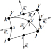Fig. 2.

Two-dimensional finite element

2.2 Three-dimensional discretization element

In order to solve the problem of determining the strength parameters of AIC constructions in a three-dimensional formulation (Fig. 3), it is proposed to use a finite element in the form of a prism with a triangular base with nodes i, j, k, m, n, p located at its vertices. In order to perform numerical integration over the volume, each such element will be mapped onto a prism, the bases of which are rectangular triangles with local coordinates 0 ≤ ξ, n ≤ 1. Vertical coordinate ζ varies within −1 ≤ ζ ≤ 1.

The column of the desired nodal unknowns of the prismatic element in the local coordinate system includes the components of the displacement vector, as well as their partial derivatives of the first order with respect to ξ,n, ξ $\underset{1 \times 72}{{V_{y}^{L}}^{T}} = {\begin{matrix} \underset{1 \times 24}{{u_{y}^{L}}^{T}} & \underset{1 \times 24}{{v_{y}^{L}}^{T}} & \underset{1 \times 24}{{w_{y}^{L}}^{T}} \end{matrix}},$ $\mathop {\left\{ {V_{y}^{L} } \right\}^{T} }\limits_{{1 \times 72}} = \left\{ {\begin{array}{*{20}c} {\mathop {\left\{ {u_{y}^{L} } \right\}^{T} }\limits_{{1 \times 24}} } & {\mathop {\left\{ {v_{y}^{L} } \right\}^{T} }\limits_{{1 \times 24}} } & {\mathop {\left\{ {w_{y}^{L} } \right\}^{T} }\limits_{{1 \times 24}} } \\ \end{array} } \right\},$ (7)

where $\underset{1 \times 9}{{q_{y}^{L}}^{T}} = {\begin{matrix} q^{i} & q^{j} & q^{k} & q_{, ξ}^{i} & q_{, ξ}^{j} & q_{, ξ}^{k} & q_{, ξ}^{m} & q_{, ξ}^{n} & q_{, ξ}^{p} \end{matrix} \begin{matrix} q_{, η}^{i} & \dots & q_{, ζ}^{p} \end{matrix}}$ $\mathop {\left\{ {q_{y}^{L} } \right\}^{T} }\limits_{1 \times 9} = \left\{ {\begin{array}{*{20}c} {q^{i} } & {q^{j} } & {q^{k} } & {q_{,\xi }^{i} } & {q_{,\xi }^{j} } & {q_{,\xi }^{k} } & {q_{,\xi }^{m} } & {q_{,\xi }^{n} } & {q_{,\xi }^{p} } \\ \end{array} \begin{array}{*{20}c} {q_{,\eta }^{i} } & \ldots & {q_{,\zeta }^{p} } \\ \end{array} } \right\}$ .

The interpolation procedure for the components of the displacement vector of a point belonging to the inner region of the prismatic finite element is determined by the expression $\begin{matrix} q = G_{1} (ξ, η) H_{1} (ς) q^{i} + G_{2} (ξ, η) H_{1} (ς) q^{j} \\ + G_{3} (ξ, η) H_{1} (ς) q^{k} + G_{1} (ξ, η) H_{2} (ς) q^{m} + \\ + G_{2} (ξ, η) H_{2} (ς) q^{n} + G_{3} (ξ, η) H_{2} (ς) q^{p} + \\ + G_{4} (ξ, η) H_{1} (ς) q_{, ξ}^{i} + G_{5} (ξ, η) H_{1} (ς) q_{, ξ}^{j} + \\ + G_{6} (ξ, η) H_{1} (ς) q_{, ξ}^{k} + G_{4} (ξ, η) H_{2} (ς) q_{, ξ}^{m} + \\ + G_{5} (ξ, η) H_{2} (ς) q_{, ξ}^{n} + G_{6} (ξ, η) H_{2} (ς) q_{, ξ}^{p} + \\ + G_{7} (ξ, η) H_{1} (ς) q_{, η}^{i} + G_{8} (ξ, η) H_{1} (ς) q_{, η}^{j} + \\ + G_{9} (ξ, η) H_{1} (ς) q_{, η}^{k} + G_{7} (ξ, η) H_{2} (ς) q_{, η}^{m} + \dots \\ \dots + G_{1} (ξ, η) H_{3} (ς) q_{, ζ}^{i} + G_{2} (ξ, η) H_{3} (ς) q_{, ζ}^{j} + \\ + G_{3} (ξ, η) H_{3} (ς) q_{, ζ}^{k} + \dots + G_{3} (ξ, η) H_{4} (ς) q_{, ζ}^{p}, \end{matrix}$ $\begin{gathered} q = G_{1} \left( {\xi ,\eta } \right)H_{1} \left( \varsigma \right)q^{i} + G_{2} \left( {\xi ,\eta } \right)H_{1} \left( \varsigma \right)q^{j} \hfill \\ + G_{3} \left( {\xi ,\eta } \right)H_{1} \left( \varsigma \right)q^{k} + G_{1} \left( {\xi ,\eta } \right)H_{2} \left( \varsigma \right)q^{m} + \hfill \\ + G_{2} \left( {\xi ,\eta } \right)H_{2} \left( \varsigma \right)q^{n} + G_{3} \left( {\xi ,\eta } \right)H_{2} \left( \varsigma \right)q^{p} + \hfill \\ + G_{4} \left( {\xi ,\eta } \right)H_{1} \left( \varsigma \right)q_{{,\xi }}^{i} + G_{5} \left( {\xi ,\eta } \right)H_{1} \left( \varsigma \right)q_{{,\xi }}^{j} + \hfill \\ + G_{6} \left( {\xi ,\eta } \right)H_{1} \left( \varsigma \right)q_{{,\xi }}^{k} + G_{4} \left( {\xi ,\eta } \right)H_{2} \left( \varsigma \right)q_{{,\xi }}^{m} + \hfill \\ + G_{5} \left( {\xi ,\eta } \right)H_{2} \left( \varsigma \right)q_{{,\xi }}^{n} + G_{6} \left( {\xi ,\eta } \right)H_{2} \left( \varsigma \right)q_{{,\xi }}^{p} + \hfill \\ + G_{7} \left( {\xi ,\eta } \right)H_{1} \left( \varsigma \right)q_{{,\eta }}^{i} + G_{8} \left( {\xi ,\eta } \right)H_{1} \left( \varsigma \right)q_{{,\eta }}^{j} + \hfill \\ + G_{9} \left( {\xi ,\eta } \right)H_{1} \left( \varsigma \right)q_{{,\eta }}^{k} + G_{7} \left( {\xi ,\eta } \right)H_{2} \left( \varsigma \right)q_{{,\eta }}^{m} + \ldots \hfill \\ \ldots + G_{1} \left( {\xi ,\eta } \right)H_{3} \left( \varsigma \right)q_{{,\zeta }}^{i} + G_{2} \left( {\xi ,\eta } \right)H_{3} \left( \varsigma \right)q_{{,\zeta }}^{j} + \hfill \\ + G_{3} \left( {\xi ,\eta } \right)H_{3} \left( \varsigma \right)q_{{,\zeta }}^{k} + \ldots + G_{3} \left( {\xi ,\eta } \right)H_{4} \left( \varsigma \right)q_{{,\zeta }}^{p} , \hfill \\ \end{gathered}$ (8)

where G₁(ξ, η)… G₉(ξ, η) are the complete polynomials of the third degree;H₁(ϛ)…H₄(ϛ) – Hermite polynomials of the third degree.

In order to solve the compatibility problem of a volumetric finite element in the form of a prism, we use the technique described in paragraph 1 above. To do this, we introduce the Lagrange multipliers at nodes 1, 2, 3 and 4, 5, 6 located in the middle of the sides of the lower side as additional nodal unknowns and upper bases respectively (Fig. 4). Thus, for the bases of the prismatic element, the following two additional conditions can be formed $\begin{matrix} λ_{1} \frac{\partial w^{1}}{\partial {\vec{n}}_{1}} + λ_{1} \frac{\partial w^{2}}{\partial {\vec{n}}_{2}} + λ_{1} \frac{\partial w^{3}}{\partial {\vec{n}}_{3}} = 0 ; \\ λ_{4} \frac{\partial w^{4}}{\partial {\vec{n}}_{4}} + λ_{5} \frac{\partial w^{5}}{\partial {\vec{n}}_{5}} + λ_{6} \frac{\partial w^{6}}{\partial {\vec{n}}_{6}} = 0, \end{matrix}$ $\begin{gathered} \lambda _{1} \frac{{\partial w^{1} }}{{\partial \overrightarrow {n} _{1} }} + \lambda _{1} \frac{{\partial w^{2} }}{{\partial \overrightarrow {n} _{2} }} + \lambda _{1} \frac{{\partial w^{3} }}{{\partial \overrightarrow {n} _{3} }} = 0; \hfill \\ \lambda _{4} \frac{{\partial w^{4} }}{{\partial \overrightarrow {n} _{4} }} + \lambda _{5} \frac{{\partial w^{5} }}{{\partial \overrightarrow {n} _{5} }} + \lambda _{6} \frac{{\partial w^{6} }}{{\partial \overrightarrow {n} _{6} }} = 0, \hfill \\ \end{gathered}$ (9)

which can be represented in matrix form $\begin{matrix} \underset{1 \times 3}{{λ}^{T}} \underset{3 \times 1}{{\frac{\partial w^{l}}{\partial {\vec{n}}_{l}}}} = \underset{1 \times 3}{{λ}^{T}} \underset{3 \times 72}{[Φ_{1}]} \underset{72 \times 1}{{V_{y}^{L}}} = 0 ; \\ \underset{1 \times 3}{{λ}^{T}} \underset{3 \times 1}{{\frac{\partial w^{S}}{\partial {\vec{n}}_{S}}}} = \underset{1 \times 3}{{λ}^{T}} \underset{3 \times 72}{[Φ_{2}]} \underset{72 \times 1}{{V_{y}^{L}}} = 0, \end{matrix}$ $\begin{gathered} \mathop {\left\{ \lambda \right\}^{T} }\limits_{{1 \times 3}} \mathop {\left\{ {\frac{{\partial w^{l} }}{{\partial \overrightarrow {n} _{l} }}} \right\}}\limits_{{3 \times 1}} = \mathop {\left\{ \lambda \right\}^{T} }\limits_{{1 \times 3}} \mathop {\left[ {\Phi _{1} } \right]}\limits_{{3 \times 72}} \mathop {\left\{ {V_{y}^{L} } \right\}}\limits_{{72 \times 1}} = 0; \hfill \\ \mathop {\left\{ \lambda \right\}^{T} }\limits_{{1 \times 3}} \mathop {\left\{ {\frac{{\partial w^{S} }}{{\partial \overrightarrow {n} _{S} }}} \right\}}\limits_{{3 \times 1}} = \mathop {\left\{ \lambda \right\}^{T} }\limits_{{1 \times 3}} \mathop {\left[ {\Phi _{2} } \right]}\limits_{{3 \times 72}} \mathop {\left\{ {V_{y}^{L} } \right\}}\limits_{{72 \times 1}} = 0, \hfill \\ \end{gathered}$ (10)

where {λ_S}^T = {λ₄ λ₅ λ₆};[Φ₁] и [Φ₂] – matrices containing form functions representing the products of the full polynomial of the third degree and Hermite polynomial of the third degree.

The conditional Lagrange functional for a prismatic finite element, taking into account (10), can be formed as follows $\begin{matrix} Π_{L} = \int_{V} {ε_{α β}^{ς}}^{T} {σ^{ε β}}^{T} d V - \int_{F} {U}^{T} {P} d V + \\ + {λ_{l}}^{T} [Φ_{1}] [T] {V_{y}^{G}} + {λ_{S}}^{T} [Φ_{2}] [T] {V_{y}^{G}}, \end{matrix}$ $\begin{gathered} \Pi _{L} = \int\limits_{V} {\left\{ {\varepsilon _{{\alpha \beta }}^{\varsigma } } \right\}^{T} \left\{ {\sigma ^{{\varepsilon \beta }} } \right\}^{T} dV - } \int\limits_{F} {\left\{ U \right\}^{T} \left\{ P \right\}dV + } \hfill \\ + \left\{ {\lambda _{l} } \right\}^{T} \left[ {\Phi _{1} } \right]\left[ T \right]\left\{ {V_{y}^{G} } \right\} + \left\{ {\lambda _{S} } \right\}^{T} \left[ {\Phi _{2} } \right]\left[ T \right]\left\{ {V_{y}^{G} } \right\}, \hfill \\ \end{gathered}$ (11)

where ${ε_{α β}^{ς}}^{T} = {\begin{matrix} ε_{11}^{ς} & 2 ε_{12}^{ς} & 2 ε_{13}^{ς} & ε_{22}^{ς} & 2 ε_{23}^{ς} & ε_{33}^{ς} \end{matrix}}, {σ^{α β}}^{T} = {\begin{matrix} σ^{11} & σ^{12} & σ^{13} & σ^{22} & σ^{23} & σ^{33} \end{matrix}} ; {V_{y}^{G}}$ $\left\{ {\varepsilon_{\alpha \beta }^{\varsigma } } \right\}^{T} = \left\{ {\begin{array}{*{20}c} {\varepsilon_{11}^{\varsigma } } & {2\varepsilon_{12}^{\varsigma } } & {2\varepsilon_{13}^{\varsigma } } & {\varepsilon_{22}^{\varsigma } } & {2\varepsilon_{23}^{\varsigma } } & {\varepsilon_{33}^{\varsigma } } \\ \end{array} } \right\},\quad \left\{ {\sigma^{\alpha \beta } } \right\}^{T} = \left\{ {\begin{array}{*{20}c} {\sigma^{11} } & {\sigma^{12} } & {\sigma^{13} } & {\sigma^{22} } & {\sigma^{23} } & {\sigma^{33} } \\ \end{array} } \right\};\left\{ {V_{y}^{G} } \right\}$ – a column of nodal unknowns of a prismatic element in global α, β, γ coordinate system; $[T]$ $\left[ T \right]$ – transition matrix from column ${V_{y}^{L}}$ $\left\{ {V_{y}^{L} } \right\}$ to column ${V_{y}^{G}}$ $\left\{ {V_{y}^{G} } \right\}$ .

Performing the minimization procedure over (11) with respect to ${V_{y}^{G}}^{T}$ $\left\{ {V_{y}^{G} } \right\}^{T}$ , ${λ_{l}}^{T}$ $\left\{ {\lambda_{l} } \right\}^{T}$ , and ${λ_{S}}^{T}$ $\left\{ {\lambda_{S} } \right\}^{T}$ , we can compose the stiffness matrix and the column of nodal forces of the prismatic finite element, standard for FEM [19–30].

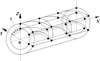Fig. 3.

Design scheme of a fragment of a pipeline using three-dimensional finite elements

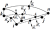Fig. 4.

Three-dimensional finite element

3 Calculation example

As an example, the problem was solved to determine the strength parameters of the design of the AIC in the form of a fragment of a cylindrical pipeline rigidly clamped at the ends and loaded with internal pressure. It should be noted that the calculated fragment of the pipeline, by its geometric characteristics, belongs to the class of thin-walled structures, to which the theory of thin shells with Kirchkoff-Love hypotheses is applicable.

The calculations were performed in two versions: in the first embodiment, a fragment of the pipeline was modeled by an ensemble of two-dimensional finite elements described in paragraph 1; in the second embodiment, a prismatic finite element was used, oriented so that the triangular bases were located on the external and internal surfaces of the pipeline, and the ribs were oriented in the direction normal to the surface of the pipeline.

The analysis of the calculated values of normal stresses on the inner and outer surfaces of the pipeline fragment showed the following. In the span section, normal stresses in the meridional and annular directions have positive values (i.e., tensile strain is observed). The numerical values of stresses in magnitude in this section turned out to be close in both versions of the calculation. In the reference section, where a moment stress state is observed, the results of the variant calculation differ significantly from each other.

Despite the stable convergence of the computational process, in both versions of the calculation, the numerical values of the meridional stresses in the second version of the calculation were underestimated by about 20% compared to the first version.

Moreover, further thickening of the grid of nodes in the second embodiment did not affect the values of the calculated meridional stresses. The values of ring stresses, which are several times less than the meridional stresses, in the second embodiment were approximately 5 and 10% higher than in the first embodiment. However, as noted above, the meridional stresses on the internal and external surfaces of the calculated structure play the most important role in the VAT picture.

Therefore, in the second version of the calculation, a sampling grid was used, which provides for dividing the cylinder in thickness not into one, but into two or even three layers of volume elements. This approach made it possible to achieve the values of meridional stresses in the reference section similar to the values of the first calculation option.

4 Conclusion

The total number of unknowns when using the second version of the calculation turned out to be about five times larger than in the first version, which makes the first option the most preferable when analyzing the SSS of agricultural structures, which can be attributed to the class of thin-walled. When determining the strength parameters of AIC objects related to structures of medium thickness and thick-walled, it is necessary to use three-dimensional prismatic finite elements of the second calculation option.

Acknowledgments

The study was carried out with the financial support of the Russian Foundation for Basic Research and the Administration of the Volgograd Region in the framework of the research project No. 19-41-340005 r_a.

References

V.A. Levin, I.S. Manuylovich, V.V. Markov, Numerical Simulation of Spinning Detonation in Circular Section Channels, Computat. Mathem. and Mathem. Phys., 56(6), 1102–1117 (2016) [CrossRef] [Google Scholar]
E.A. Storozhuk, I.S. Chernyshenko, A.V. Yatsura, Stress-Strain State Near a Hole in a Shear-Compliant Composite Cylindrical Shell with Elliptical Cross-Section, Int. Appl. Mechan., 54(5), 559–567 (2018) [CrossRef] [Google Scholar]
I.B. Badriev, V.N. Paimushin, Refined Models of Contact Interaction of a Thin Plate with Positioned on Both Sides Deformable Foundations, Lobachevskii J. of Mathem., 38(5), 779–793 (2017) [CrossRef] [Google Scholar]
I.B. Badriev, M.V. Makarov, V.N. Paimushin, Contact Statement of Mechanical Problems of Reinforced on a Contour Sandwich Plates with Transversally-Soft Core, Russ. Mathem., 61(1), 69–75 (2017) [CrossRef] [Google Scholar]
A.S. Solodovnikov, S.V. Sheshenin, Numerical Study of Strength Properties for a Composite Material with Short Reinforcing Fibers, Moscow Univer. Mechan. Bull., 72(4), 94–100 (2017) [Google Scholar]
V.N. Shlyannikov, A.P. Zakharov, A.V. Tumanov, Nonlinear fracture resistance parameters for elements of aviation structures under biaxial loading, Russ. Aeronaut., 61(3), 340–346 (2018) [CrossRef] [Google Scholar]
F. Aldakheel, B. Hudobivnik, P. Wriggers, Virtual selection of phase definitions, Int. J. for Multiscale Computat. Engineer. (2018) [Google Scholar]
L.U. Sultanov, Analysis of Finite Elasto-Plastic Strains. Medium Kinematics and Constitutive Equations, Lobachevskii J. of Mathem., 37(6), 787–793 (2016) [CrossRef] [Google Scholar]
R.A. Kayumov, Postbuckling Behavior of Compressed Rods in an Elastic Medium, Mechan. of Solids, 52(5), 575–580 (2017) [Google Scholar]
K.-J. Bathe, Finite Element Procedures (Prentice Hall, Englewood Cliffs, 1996) [Google Scholar]
O.C. Zienkiewicz, R.L. Taylor, J.Z. Zhu, The Finite Element Method: Its Basis and Fundamentals (Butter-worth-Heinemann, United Kingdom, 2013) [Google Scholar]
J.T. Oden, Finite Elements of Nonlinear Continua (McGraw-Hill, New York, 1971) [Google Scholar]
A.M. Belostotsky, S.B. Penkovoy, S.V. Scherbina, P.A. Akimov, T.B. Kaytukov, Correct Numerical Methods of Analysis of Structural Strength and Stability of High-Rise Panel Buildings, Part 1: Theoretical Foundations of Modelling, Key Engineering Materials, 685, 217–220 (2016) [Google Scholar]
E. Artioli, L.B.D.D. Veiga, C. Lovadina, E. Sacco, Arbitrary order 2d virtual elements for polygonal meshes: Part I, elastic problem, Computat. Mechan., 60, 355–377 (2017) [CrossRef] [Google Scholar]
E. Artioli, L.B.D.D. Veiga, C. Lovadina, E. Sacco, Arbitrary order 2d for polygonal meshes: Part II, inelastic problem, Computat. Mechan., 60, 643–657 (2017) [CrossRef] [Google Scholar]
P. Wriggers, W. Rust, B. Reddy, A virtual element method for contact, Computat. Mechan., 58, 1039–1050 (2016) [CrossRef] [Google Scholar]
Ren Hui, Fast and robust triangular elements for thin plates/shells, with large deformations and large rotations, Trans. ASME. J. Comput. and Nonlinear Dyn., 10(5), 051018/1-051018/13 (2015) [Google Scholar]
Y.V. Klochkov, A.P. Nikolaev, O.V. Vakhnina, T.A. Kiseleva, Using the Lagrange multiplexes in the triangles of the interregolation of displacements, J. of Applied and Industr. Mathem., 11(4), 535–544 (2017) [CrossRef] [Google Scholar]
L.P. Zheleznov, V.V. Kabanov, D.V. Boiko, Elliptical Cylindrical Composite Shells under Torsion and Internal Pressure, Russ. Aeronaut., 61(2), 175–182 (2018) [Google Scholar]
L.P. Zheleznov, V.V. Kabanov, D.V. Boiko, Nonlinear Deformation and Stability of Discretely Reinforced Elliptical Cylindrical Shells under Transverse Bending and Internal Pressure, Russ. Aeronaut., 57(2), 118–126 (2014) [CrossRef] [Google Scholar]
V.P. Agapov, R.O. Golovanov, K.R. Aidemirov, Calculation of Load-Bearing Capacity of Prestressed Reinforced Concrete Trusses by the Finite Element Method, IOP Conf. Ser. Earth and Environmental Sci., 90, 012018 (2017) [Google Scholar]
Yu.V. Klochkov, A.P. Nikolaev, T.A. Kiseleva, S. S. Marchenko, Comparative analysis of the results of finite element calculations based on an ellipsoidal shell, J. of Machin. Manufact. and Reliab., 45(4), 328–336 (2016) [CrossRef] [Google Scholar]
Yamashita Hirok, Valkeapaa Antti I., Jayakumar Paramsothy, Syqiyama Hiroyuki, Continuum mechanics based bilinear shear deformable shell element using absolute nodal coordinate formulation, Trans. ASME. J. Comput. and Nonlinear Dyn., 10(5), 051012/1-051012/9 (2015) [Google Scholar]
Nhung Nguyen, Anthonym Waas, Nonlinear, finite deformation, finite element analysis, ZAMP. Z. Angew. math. and Phys., 67(9), 35/1-35/24 (2016) [Google Scholar]
Zhen Lei, F. Gillot, Jezeguel, Development of the mixed grid isogeometric Reissner-Mindlin shell: quadrate basis and modified quadrature, Int. J. Mech., 54, 105–119 (2015) [Google Scholar]
A. Javili, A. Mc Bride, P. Steinmann, B.D. Reddy, A curvilinear-coordinate based finite elemental methodology, Comput. Mech., 54(3), 745–762 (2014) [Google Scholar]
He Xiaocong, Torsional analysis of free vibration of adhesively bonded single-lap joints, Int. J. Adhes. and Adnes., 48, 59–66 (2014) [CrossRef] [Google Scholar]
S.N. Yakupov, N.M. Yakupov, Thin-Layer Films and Coatings, Mechan. of Solids, 857(1), 012056 (2017) [Google Scholar]
A.M. Belostotsky, P.A. Akimov, I.N. Afanasyeva, T. B. Kaytukov, Contemporary Problems of Numerical Modelling of Unique Structures and Buildings, Int. J. for Computat. Civil and Struct. Engineer., 13(2), 9 (2018) [Google Scholar]
Yu.V. Klochkov, A.P. Nikolaev, T.A. Kiseleva, S.S. Marchenko, Comparative analysis of the results of finite element calculations based on an ellipsoidal shell, J. of Machin. Manufact. and Reliab., 45(4), 328–336 (2016) [CrossRef] [Google Scholar]

All Figures

	Fig. 1. Design scheme of the fragment of the pipeline using two-dimensional finite elements
In the text

	Fig. 2. Two-dimensional finite element
In the text

	Fig. 3. Design scheme of a fragment of a pipeline using three-dimensional finite elements
In the text

	Fig. 4. Three-dimensional finite element
In the text

Current usage metrics show cumulative count of Article Views (full-text article views including HTML views, PDF and ePub downloads, according to the available data) and Abstracts Views on Vision4Press platform.

Data correspond to usage on the plateform after 2015. The current usage metrics is available 48-96 hours after online publication and is updated daily on week days.

Initial download of the metrics may take a while.