| Issue |
BIO Web Conf.
Volume 68, 2023
44th World Congress of Vine and Wine
|
|
|---|---|---|
| Article Number | 01022 | |
| Number of page(s) | 9 | |
| Section | Viticulture | |
| DOI | https://doi.org/10.1051/bioconf/20236801022 | |
| Published online | 06 December 2023 | |
Satellite and UAV-based anomaly detection in vineyards
1 Spin.Works S.A., Av. da Igreja 42, 6º, 1700-239 Lisboa, Portugal
2 Sogrape Vinhos, S.A., Rua 5 de outubro 4527, 4430-809 Avintes, Portugal
Abstract
One of the most frequent, most expensive and potentially more impactful tasks in crop management is surveying and scouting the fields for problems in crop development. Any biotic / abiotic stress undetected becomes a bigger problem to solve later, with a potentially cascading effect on yield and/or quality and, subsequently, crop value. For annual crops (such as corn, soy, etc.) this can be solved in a cost-effective way with Sentinel data. For permanent crops planted in rows (such as vineyards), the interference from the inter-row makes it much more challenging. Under a contract for the European Space Agency (ESA), Spin.Works has been developing an early anomaly detection system based on fusion of Sentinel-2 and UAV imagery, targeting an update rate of 5 days. The early anomaly detection is applied to vineyards, particularly, for nutrient and water stresses. The early anomaly detection system is integrated into Spin.Works’ MAPP.it platform and its development is being carried out in close cooperation with the internal R&D group of Sogrape Vinhos, Portugal's largest winemaker and a long-standing MAPP.it user.
© The Authors, published by EDP Sciences, 2023
 This is an Open Access article distributed under the terms of the Creative Commons Attribution License 4.0, which permits unrestricted use, distribution, and reproduction in any medium, provided the original work is properly cited.
1 Introduction
Within the large scope of remote sensing-based anomaly detection in vineyard development, the study focuses on two - water and nutrient - stresses and this paper presents the common approach to both and details the preliminary results for the former.
1.1 Satellite vs. UAV
We shall refer to “remote sensing” in its wider scope encompassing not only satellite sourced imagery, but also that obtained with aircraft and unmanned aerial vehicles (UAV).
The key variables when comparing data sources for vineyard management applications are: ground sampling distance (or spatial resolution), bands acquired and cost. Free satellite multispectral imagery such as that provided by the European Union Copernicus Programme (through Sentinel-2A and 2B satellites) starts at 10 m/pixel and has more bands than the typical UAV image. Paid satellite imagery starts at ~30 cm/pixel, requires tasking a satellite and implies a minimum area, which drives up costs for small areas such as vineyards. Cost is a relevant variable not only for a cost-benefit analysis in the context of user adoption but is also closely related with temporal resolution. The cost of each UAV image limits the number of images through the season, whereas free satellite data is available every 5 days. In general terms and taking cost into account, UAV imagery has an advantage in spatial resolution, while free satellite imagery from Copernicus has an advantage in temporal resolution (i.e., revisit times).
For permanent crops planted in rows (such as vineyards), addressing inter-row interference is important to ensure accurate and reliable remote sensing data. Inter-row interference or contamination occurs when the sensor used for remote sensing captures the reflectance not only from the target crop, but also from the surrounding inter-row spaces. This happens when the width of the rows is smaller than the spatial resolution.
1.2 Literature review
Studies comparing UAV and free satellite imagery from Sentinel-2 suggest that satellite imagery cannot be directly used to reliably describe vineyard variability due to the “contribution of the inter-row surfaces” [2]. Good correlations were detected between unfiltered Sentinel-2 and UAV NDVI [3], which only means that the contribution of the inter-row surfaces is similarly represented in both images. In vineyards without inter-row vegetation, in plots larger than 0.5 ha, and when border pixels are removed, Sentinel-2 can reliably be used to map variability [4].
In [5] “a thermal-based multi-sensor data fusion approach [was used] to generate weekly total actual ET [Evapotranspiration] (ETa) estimates at 30 m spatial resolution, coinciding with the resolution of the Landsat reflectance bands. […] (ETc) [was] defined with a vegetative index (VI)-based approach. To test capacity to capture stress signals, the vineyard was sub-divided into four blocks with different irrigation management strategies and goals, inducing varying degrees of stress during the growing season. It concludes that “[r]esults indicate derived weekly total ET from the thermal-based data fusion approach match well with observations. The thermal-based method was also able to capture the spatial heterogeneity in ET over the vineyard due to a water stress event imposed on two of the four vineyard blocks. This transient stress event was not reflected in the VI-based ETc estimate, highlighting the value of thermal band imaging.” 5 makes no reference to the inter-row cover (grass, cover crop, bare soil, etc.).
The vineyard used for the study in 6 has the inter-rows maintained vegetation-free and it is concluded that “[t]he RS-PM models [Sentinel-2 based] outperform the METRIC and TSEB-PT models [Landsat 7 and 8], especially in the instantaneous and daily time scales where RS-PM models have the lowest root mean square error (RMSE) and the highest Wilmott agreement index”. It demonstrates “that RS-PMS model is suitable to assess water consumption and irrigation management, since it is possible to estimate the actual Kc of the vineyard with the actual modelled ET (Kc PMS), which is one of the criteria used in irrigation management. Thus, on average the Kc PMS is biased by 9% compared to the Kc estimated with data from the Eddy covariance system (Kc EC). This is relevant taking into account it was found that during the two evaluated seasons, the vineyard’s Kc was below of the 0.5 target Kc, equivalent to 0.33 in S1 (2017-2018) and 0.34 in S2 (2018-2019), representing a 32% lower than planned.”
The test site in 7 involves “annual cover-cropping with oats (45%), barley (45%), and mustard (10%)” and concludes that the “study indicates that limited deployment of sUAS [Drones] can provide important estimates of uncertainty in EOS [Earth Observation-based] ET estimations for larger areas and to also improve irrigation management at a local scale.” It is noted that “The EOS ET estimates are most similar to the sUAS ET when bare soil is masked out, especially during the peak of the season when the canopy is fully grown and covers most of the field area. It seems likely that the lower spatial resolution from EOS platforms leads to an overestimation of ET for vineyards as the peak ET from the canopy gets generalized for the entire cell area, which in reality contains areas with much less ET like we can observe with the sUAS imagery.”
In 8 the study monitored thirty six plots of about 1 ha with the majority with bare soil (67%) and were monitored for a period of three years (2018-2020). In each vine plot, from one to six subplots were assigned for data acquisition and the stem water potential was measured on several vine roots (rSWP). The authors assessed four different machine learning algorithms on predicting vine water status through the Sentinel-2 imagery and compared them with 7 different vegetation indices. The authors concluded that the linear regression model yielded promising results to predict stem water potential from different years, grape varieties and grass management. It is noted, however, that it was necessary “to take into account the particularity of vine management in row and not to forget the potential impact of grass cover or soil management/composition to the result interpretation”. The study highlights that “the model performs better when only plots without grass in the inter-row are considered (R2 = 0.48 and RMSE = 0.24 vs. R2 = 0.40 and RMSE = 0.26). However, […] the results when also considering plots with grass show that only few points deviate from the trend. It can be explained by the fact that in Mediterranean region the vegetation in the inter-row is not always well developed especially in the middle of summer.”
1.3 Current approaches and their limitations
The current state-of-the-art in remote sensing for precision viticulture in row crops relies on very high spatial resolution (~10 cm) UAV multi-spectral imaging [9] and emerging open-data satellite-based approaches are limited by inter-row interference and mostly address variability mapping and water status. Furthermore, UAV-based solutions suffer from low temporal resolution due to cost and open-data satellite-based solutions (Sentinel and Landsat) suffer from low spatial resolution.
2 Materials and methods
2.1 Study area
The complete study area comprises estates in six Portuguese wine regions (Vinho Verde, Douro, Bairrada, Dão, Bucelas and Alentejo). Ultimately the study area is limited by the availability of data, in particular by the intersection between the available field data and Very High Resolution (VHR) remote sensing data. The “VHR” terminology is used as an origin-independent generalisation. To maximise the available data for modelling purposes and instead of limiting the choice to imagery strictly obtained with UAV, we also use satellite, if it is of very high resolution.
The study area encompasses 9 vineyard holdings, totalling 580 hectares of vineyard area. The vineyards are planted with more than 60 different grape varieties and are typical of very different situations. More than 300 hectares are in mountain areas, displaying steep slopes, high slope aspect variation and diverse vineyard structural systems. Overall, the properties present a very rich and diverse sample in terms of characteristics, structures and complexities.
The preliminary results presented in Section 3 refer to the water stress case and therefore the study area is a subset of 3 estates for which measurements of pre-dawn leaf water potential are available. These are located in the Douro and Alentejo regions: DS3, DS4 and A1.
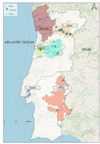 |
Figure 1. Study area. Studied estates are marked with blue pins. |
Primary locations of the Estates.
Available field and VHR images for the study.
2.2 Dataset
The dataset consists of 5 main data types: field, weather and topographic data and Very High Resolution and Medium Resolution (MR) imagery.
2.2.1 Very high resolution imagery
VHR imagery (typically better than ~1 m/pixel) can be acquired by satellites, (manned) aircraft or UAVs and, for modelling purposes, their origin is not relevant. For inference and future operational purposes however, it shall be limited to UAV due to cost.
The use of VHR satellite imagery considers a trade-off between spatial resolution, availability, and access costs. Through the ESA Third Party Missions programme (TPM) we have selected SPOT, Pleiades, and Pleiades Neo (PNEO) as valuable options to explore. These missions provide common Panchromatic, Blue, Green, Red and Near Infra-Red bands (additionally Deep Blue and Red-Edge for the PNEO), within a spatial resolution range of 1.50, 0.50, and 0.30 m respectively. Nevertheless, for the target study area only lower spatial resolution images (SPOT) were available.
UAV (5-10 cm/pixel) multi-spectral imagery used is gathered at low altitude (typically <120 m above-ground level - AGL), using micro-UAV platforms and COTS cameras. Typical platforms used are Spin.Works’ own S20 fixed-wing UAV, Wingtra WingtraOne or several DJI multi-rotor UAVs, the latter typically used for coverage of smaller areas. Red, Green, Blue, Red Edge and Near Infra-Red (NIR) bands are available from cameras like the Micasense RedEdge MX, RedEdge-P or Altum-PT (the latter adding a low-resolution thermal band).
Available VHR imagery (1Field outside the study area used solely for data fusion testing).
2.2.2 Medium Resolution imagery
In this study we use medium resolution (10-60 m/pixel) multi-spectral imaging sourced from Copernicus, the European Union Earth Observation programme. The images are obtained by the Sentinel-2 satellites, which provide global land coverage every five days over any given location.
Sentinel-2 images were acquired and processed in the L2A levels from the sentinel hub API. The L2A level is atmospherically corrected and complemented with a cloud mask. The images were selected according to two criteria: i) no cloud covering over the target estates and ii) a maximum of 5 days between the date image and the water status measurement (when applicable). These multi-spectral optical images include 13 spectral bands in the visible, near infra-red (NIR) and short-wave infrared (SWIR) spectral regions. 10 bands were used in this study with a spatial resolution of 10 m and 20 m (B2, B3, B4, B5, B6, B7, B8, B81, B11, B12). In total, 51 images were available from June to September. The Sentinel-2 bands are subsequentially merged together in one multi-spectral image. The pixel values of each band have been divided by 10,000 in order to convert them to reflectance.
2.2.3 Field data
For the purpose of this study Sogrape granted access to their available field data relevant for both the water and nutrient stress cases. The dataset comprises phenological data of each cultivar, weather data, pre-dawn leaf water potential, foliar and soil analysis, phyto-pharmaceutical and fertilizer applications of each estate for 2022.
Pre-dawn leaf water potential (ψ_PD) was obtained in weekly measurements between June and September of 2022 for three estates (DS3, DS4 and A1). The measurements were carried out before dawn using a pressure chamber. In total 420 readings pre-dawn leaf water potential are available for 2022, divided as per the table below.
Soil and leaf analyses for 2021 (D1, DS3, DS4, VV1, BA3, A1) coupled with daily records of phyto-pharmaceutical and fertilizer applications (DS3, DS4, VV1, BA3, D1, A1) for 2022 are available. Soil and leaf analyses contain existing macronutrients (N,P,K,Ca,Mg), micronutrient (Bo, Cu, Zn, Fe, Mn), cation exchange capacity (Ca2+, Mg2+, K+,Na+, Al+3), soil metal content, pH levels, apparent electrical conductivity, organic matter, nutrient ratios (Dris analysis), soil structure and texture. The applications logs have the type of application coupled with the amount (fertilizer, pyto-pharmaceuticals), the parcel and the day of the application.
Pre-dawn leaf water potential measurement details broke down by estate.
2.2.4 Weather data
Weather data comprises records of temperature, rainfall, incident radiation, relative humidity, wind direction and velocity, at 15 min intervals. DS3, DS4 and A1 were continuously monitored by a total of 5 weather stations: 2 at DS3, 1 at DS4 and 2 at A1.
2.2.5 Topographic data
For DS3, DS4 and A1 estates, high resolution Digital Surface Models (DSM), with 15 x 15 cm pixel resolution are available. The DSM was converted to a Digital Elevation Model (DEM), by removing the above-ground features with the Metashape pro software. Then, the DEM was resampled to a more usable 2 x 2 m resolution.
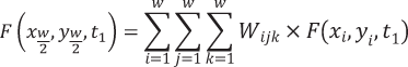
2.3 Data fusion pipeline
2.3.1 Data fusion
Data fusion involves the fusion of remote sensing products from satellites and aerial imagery. The main goal for this module is to use data fusion to produce a product with both high temporal and high spatial resolution by combining a free high temporal, coarse resolution product (Sentinel-2) with commercial very fine resolution data with low temporal resolution due to costs (drone aerial imagery or VHR commercials satellite imagery, such as SPOT, Pleiades or Pleiades NEO).
STARFM (Spatial and Temporal Adaptive Reflectance Fusion Model) is a widely used data fusion algorithm for combining multispectral satellite images acquired at different spatial and temporal resolutions. In this study, we are considering this approach as the baseline model for data fusion.
The algorithm in the equation below assumes that the fine resolution surface reflectance (F) at the prediction date (t1) can be retrieved by using information from a pair of a fine resolution image (F) and a coarse resolution image (C) at a date preceding/following the date of prediction (t0) and a coarse resolution image (C) at the date of prediction (t1). Supposing the ground coverage type and system errors at pixel (xi,yi) do not change over reference date (t0) and prediction date (t1), the fine resolution reflectance values can be estimated by:
 (1)
(1)
This ideal situation cannot be satisfied since coarse observation (Sentinel-2) is not a homogeneous pixel and may include mixed land-cover types when considered at the fine spatial resolution of the Drone imagery or VHR satellites; land cover may change from one type to another during the prediction period and land-cover phenology or solar geometry bidirectional reflectance distribution function (BRDF) changes will change the reflectance from reference date to prediction date. Therefore, the authors proposed to introduce additional information from neighbouring pixels, by using a weighted function:
 (2)
(2)
where (w) is the search window size and (xw/2,yw/2) is the central pixel of the moving window. (n) is the number of input reference pairs. The weighting function determines how much each neighbour pixel contributes to the estimated reflectance of the central pixel and comprises the contributions from the spectral distance between fine and coarse images on reference date, temporal distance between the coarse images on reference and prediction date and spatial distances to the central pixel.
2.3.2 Implementation
The implementation of the data fusion pipeline involves several pre-processing steps. First, Sentinel-2 data is masked with drone imagery bounds, then Sentinel images are re-sampled to the target high resolution. Next, all images (Sentinel-2 and drone) are co-registered according to the same reference, then vegetation indexes are calculated and finally those products become inputs to the data fusion algorithm.
The first step consists in cropping the region of interest from the Sentinel-2 products according to the polygon available for the drone imagery, as well as the most similar bands.
The second step consists in re-sampling both products to the target resolution. The drone orthomosaic is generated and resampled to the target resolution of 1.25m. Sentinel-2 bands Blue (B02), Green (B03), Red (B04), Red Edge (B05) and NIR (B08) are re-sampled also to 1.25 m GSD using both nearest-neighbour and bicubic interpolation.
The third step is the co-registration of all the bands from the two sources by applying a parametric image alignment technique using enhanced correlation coefficient maximization 12. This method requires the pre-computing of the mean gradient image from every RGB composite Sentinel-2 image along each subject year in order to use as a reference for subsequent satellite imagery registration. For each sample from each subject year, a gradient image is produced from its RGB composite and compared with the previously computed reference image, ultimately obtaining an affine matrix containing the estimated horizontal and vertical shifts. In the end, each sample’s band is subject to an affine transform using the estimated shifts, resulting a well registered collection for each year.
The last pre-processing step is the calculation of the vegetation indexes.
 |
Figure 2. Data fusion pipeline. |
2.4 Estimation of water status
2.4.1 Problem definition
Plant water status is assessed through the Pre-dawn leaf water potential (ψ_PD). From a Machine Learning standpoint, we opted to first address this problem as a regression problem, i.e., where the goal is to obtain a model that can estimate (or predict) the actual ψ_PD from observable parameters.
2.4.2 Data pre-processing
Since the weather stations presented similar patterns, it was decided to average the climatic data for each estate (Fig. 3). Afterwards, the weather datasets were converted into daily records, with minimum, mean and maximum for each day. From this information, other parameters relevant towards the plant water status were calculated, such as vapour pressure deficit, evapotranspiration, heat-hours, growing degree-days and sunlight hours over three and five days.
Since topography has a decisive influence on water distribution, several primary and secondary topographic parameters were extracted from the DEM to characterize the three study areas. Deviation from mean elevation characterises the relative elevation with respect to its surroundings; flow accumulation and Wetness Index indicate the propensity for moisture and water accumulation; aspect, eastness and northness are metrics which indicate the terrain orientation; planar, profile, tangential and minimum curvature characterise the different types of terrain curvature; and ruggedness; slope represents the rate of change of elevation; ruggedness represents the variation of slope.
From the Sentinel-2 data, the images were selected according to the criteria used by 9: i) no cloud cover on the plots and ii) a maximum of 5 days between the image date and the ψ_PD measurements. Several vegetation indices related with water stress were identified from existing bibliography Table 5).
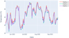 |
Figure 3. DS3 and DS4 temperature data. |
Vegetation indices considered.
2.4.2 Data preparation
To prepare the dataset for a machine learning problem, each entry of the measured output yi (ψPD) was matched with the corresponding features Xij, comprising all weather, topographic and remote sensing data. The entire dataset (outputs and features) was scaled using the Sklearn Standard Scaler.
Investigation of the original ψPD distribution (Fig. 4) revealed a skew to the right, which can be balanced by a logarithmic correction. In order to manage the complexity of the obtained models (even if at the expense of the design space size), three different distributions of ψPD were assessed: i) original distribution ψPD ii) standardised distribution resulting from the Sklearn Standard Scaler and ψPD, std iii) standardised combined with logarithmic correction ψPD, log.
From the weather, remote sensing and topography data, a total of 113 different features were derived. In order to reduce the data complexity and processing time, 4 feature reduction methods were used, using a combination of the python Select Kbest method, Variance Inflation Factor and expert knowledge. The result was 4 sets of features: 1) feature set S1 chosen with Select Kbest only, 2) feature set S2 chosen with Select Kbest plus Variance Inflation Factor, 3) feature set S3 chosen strictly through expert knowledge and 4) feature set S4 chosen using a combination of expert knowledge and Variance Inflation Factor.
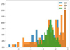 |
Figure 4. Distribution of pre-dawn leaf water potential for the three estates. |
2.4.3 Approach to regression problem
In order to estimate (or predict) the actual ψPD multiple supervised regression algorithms were tested (Table 6).
These 6 algorithms were evaluated using 4 feature sets (S1, S2, S3 and S4) and the 3 different ψPD distributions (ψPD, ψPD.std and ψPD, log).
Each different feature set and ψPD distribution combination was aggregated into a dataset, which in turn were split into 10 folds (k = 10) using a stratified shuffle split (following the standard 80/20 test/train split). This approach was followed due to the limited availability of ψPD measurements, which unbalanced the train and test sets resulting in inaccurate validation results. The stratified shuffle split was employed to ensure a stable sampling process. To control the data distribution, a 10-bin stratification process was implemented, ensuring that each bin contained samples from all ψPD throughout the year.
Then, the best model for the combined estates was identified, and tested individually in each estate for its generalization capability. Afterwards, the model that best fit the specific conditions of each estate was identified.
Details on the algorithms used.
3 Results and Discussion
The next sections discuss and document the study’s preliminary results on remote sensing-based detection of water stress throughout the growing season.
3.1 Data fusion: Preliminary results
Preliminary results using the STARFM algorithm for 5 dates are evaluated by photo-interpretation and using 2 preliminary image similarity metrics: the root mean square error (RMSE) and Pearson correlation coefficient between the predicted and observed vegetation indexes.
Each figure contains in the first line the Sentinel-2 and Drone NDVI at the reference date (T0) and at the second line the Sentinel-2, drone and fusion NDVI at the prediction date (T1). The Fusion T1 product is originated from Sentinel T0, Drone T0 and Sentinel-2 T1 using STARFM. Drone T1 is considered the ground truth data for the prediction date.
The 5 estimated fusion products are compared using RMSE and Pearson Correlation with the 5 drone product with similar dates. These results are represented in Figure 6 by the blue lines. The green line is the comparison between the bi-cubic interpolated Sentinel-2 products against the drone ground truth at similar dates and the orange lines represent the comparison of the first drone image with the next ones. The last 2 products are the baseline, available when data fusion does not exist.
In general, one can see that the fusion products outperform the existing baselines which is a very promising result. The second date however, requires further investigation given its behaviour against the trend of the posterior dates.
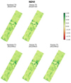 |
Figure 5. Sample NDVI from Sentinel, drone and fusion. |
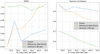 |
Figure 6. Data Fusion Metrics. Left – Root Mean Squared Error. Right – Pearson Correlation. |
3.2 Estimation of water status: Preliminary results
3.2.1 Best global and local models
Preliminary results modelling the ψ_PD for the 3 estates combined indicates that the best combination of algorithm, feature set and distribution is the S2, with a logarithmic distribution using the Extra Trees Regressor (ExT), yielding an R2 of 0.538 (Table 7). The sensitivity to different features and distribution combinations is not negligible, but also not very high with all above an R2 of 0.4 and 4 out of 12 higher than 0.5.
The Support Vector Regression (SVR-poly) is the second-best algorithm and shows similar sensitivity to the Extra Trees Regressor (ExT).
Surface Vector regression using a radial kernel and Linear Regression models never outperform the other 5 algorithms. Their results were thus omitted from the summary table to facilitate the reading.
Table 8 below shows the results for the best global model and compares it against: a) those for each estate in isolation using the same algorithm-features-distribution combination; and b) with the results for the best local models for each estate.
The results in DS3 and A1 under-perform when compared with the global model trained with all 3 estates. Since DS3 and DS4 share the same grape variety, as well as several climatic and topographic similarities due to being in proximity, we were expecting closer results. The under performance of the best model in A1 (R2 = 0.4) could be explained by its approximately normal distribution (Fig. 4), which does not require a logarithmic correction.
The results from the best models obtained for each individual estate, show that estate A1 was the only one to have better results without normalising the ψPD, which reinforces the previous explanation. One also verifies that, as expected, the R2 values for all 3 best local models is either equal or higher than that of the best global model.
Best performing algorithms for the 3 estates combined, with different combinations between feature sets, and ψ_PD distributions.
Summary of best global and local models.
3.2.2 Feature analysis
From the best global model, the feature importance analysis (Fig. 7) reveals that both the weather, topography and remote sensing information appear to positively contribute to model the ψPD, with the exception to the Moisture stress index (Msi). Topography and climate data were determinant in the ψPD prediction, with the wetness index, aspect, the mean maximum temperature of the last 5 days (Temp_max_5d) and the total hours of sun per day (HS_sum_dia) being the ones with most impact.
The remote sensing variables were not among the most relevant features but presented a consistent performance. Contrary to what would be expected, the SWIR band known to be closely related to water stress [8,20], was negatively impacting the results, with an improvement in the model performance when MSI was permuted out. A possible explanation for this might lie in the ground sampling distance of the Sentinel-2’s SWIR band, which at this preliminary stage does not yet benefit from any fusion with UAV data and thus does not address inter-row interference.
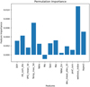 |
Figure 7. Feature importance calculated using the permutation importance method. |
4 Conclusion
Preliminary results were obtained for independent developments of UAV-Satellite data fusion and satellite-based pre-dawn leaf water potential estimation.
Satellite-UAV data fusion using the baseline STARFM algorithm yielded promising results both qualitatively as well as quantitatively as measured by RMSE and Pearson correlation.
Pre-dawn leaf water potential estimation was treated as a regression problem. Seven different algorithms, 4 feature sets and 3 measurement distributions were combined and applied to 3 different estates both in isolation and as whole. From this design space the best overall global model was the one based on Extra Trees Regression yielding an R2 of 0.53 and RMSE of 1.2 bar. The model was trained and tested on 3 estates with 2 different varieties, located in 2 different wine regions in Portugal with data from a single growing season.
With the caveat of only considering one growing season at this stage, these results suggest an improvement upon the work documented in 8, in which an R2 of 0.4 was reached when all plots were considered. In 8 removing the inter-row effect managed to improve the results to an R2 of 0.48, which suggests that doing so through satellite-UAV data fusion as proposed here, could allow the model to better leverage the remote sensing data and thus improve its ψPD estimates.
References
- Matese et al., Intercomparison of UAV, aircraft and satellite remote sensing platforms for precision viticulture. Remote Sensing 7(3), 2971–2990 (2015) [Google Scholar]
- A. Khaliq, et al., Comparison of Satellite and UAV-Based Multispectral Imagery for Vineyard Variability Assessment, Remote Sensing 11(4), 436 (2019) https://doi.org/10.3390/rs11040436 [CrossRef] [Google Scholar]
- L. Pastonchi, et al., Comparison between satellite and ground data with UAV-based information to analyse vineyard spatio-temporal variability, Oeno One 54, 4 (2020), https://doi.org/10.20870/oeno-one.2020.54.4.4028 [Google Scholar]
- M. Sozzi, et al., Comparing vineyard imagery acquired from Sentinel-2 and Unmanned Aerial Vehicle (UAV) platform, Oeno One 54, 2 (2020) https://doi.org/10.20870/oeno-one.2020.54.1.2557 [Google Scholar]
- K. R. Knipper, et al., Using High-Spatiotemporal Thermal Satellite ET Retrievals for Operational Water Use and Stress Monitoring in a California Vineyard, Remote Sensing 11(18), 2124 (2019) https://www.mdpi.com/2072-4292/11/18/2124?type=check_update&version=2 [CrossRef] [Google Scholar]
- V. Garcia-Gutiérrez, et al., Evaluation of Penman-Monteith Model Based on Sentinel-2 Data for the Estimation of Actual Evapotranspiration in Vineyards, Remote Sensing 13(3), 478 (2021) https://www.mdpi.com/2072-4292/13/3/478?type=check_update&version=4 [CrossRef] [Google Scholar]
- M. Kalua, et al., Remote Sensing of Vineyard Evapotranspiration Quantifies Spatiotemporal Uncertainty in Satellite-Borne ET Estimates, Remote Sensing 12(19), 3251 (2020) https://www.mdpi.com/2072-4292/12/19/3251?type=check_update&version=1 [CrossRef] [Google Scholar]
- E. Laroche-Pinel, et al., Towards Vine Water Status Monitoring on a Large Scale Using Sentinel-2 Images, Remote Sensing 13(9), 1837 (2021) https://www.mdpi.com/2072-|4292/13/9/1837?type=check_update&version=1 [CrossRef] [Google Scholar]
- João Araújo, et al., Innovation co-development for viticulture and enology: novel tele-detection web-service fuses vineyard data, BIO Web Conf. 56, 43rd World Congress of Vine and Wine, 2023 https://www.bio-conferences.org/articles/bioconf/full_html/2023/01/bioconf_oiv2022_01006/bioconf_oiv2022_01006.html [Google Scholar]
- J.B. MacQueen, Some Methods for classification and Analysis of Multivariate Observations, Proceedings of 5th Berkeley Symposium on Mathematical Statistics and Probability, University of California Press 1, 281-297 MR 0214227. Zbl 0214.46201. Retrieved 2009-04-07. [Google Scholar]
- M. Kazmierski, et al., Temporal stability of within-field patterns of NDVI in non-irrigated Mediterranean vineyards Oeno One 45(2), 61–73 (2011) [CrossRef] [Google Scholar]
- Georgios D. Evangelidis, Emmanouil Z. Psarakis, Parametric image alignment using enhanced correlation coefficient maximization Pattern Analysis and Machine Intelligence, IEEE Transactions on 30(10), 1858–1865 (2008) [CrossRef] [PubMed] [Google Scholar]
- Cohen, Y., et al. Can time series of multispectral satellite images be used to estimate stem water potential in vineyards? Precision agriculture’19. Wageningen Academic Publishers, 2019. 1-5. https://doi.org/10.3920/978-90-8686-888-9_55 [Google Scholar]
- Tang, Zhehan, et al. Vine water status mapping with multispectral UAV imagery and machine learning Irrigation Science 40, 4-5 (2022) https://doi.org/10.1007/s00271-022-00788-w [Google Scholar]
- Romero, Maria, et al. Vineyard water status estimation using multispectral imagery from an UAV platform and machine learning algorithms for irrigation scheduling management Computers and electronics in agriculture 147, 109-117 (2018) https://doi.org/10.1016/j.compag.2018.02.013 [CrossRef] [Google Scholar]
- Poblete, Tomas, et al. Arti7ficial neural network to predict vine water status spatial variability using multispectral information obtained from an unmanned aerial vehicle (UAV) Sensors 17(11), 2488 (2017) https://doi.org/10.3390/s17112488 [CrossRef] [PubMed] [Google Scholar]
- Cogato, Alessia, et al. Evaluating the Spectral and Physiological Responses of Grapevines (Vitis vinifera L.) to Heat and Water Stresses under Different Vineyard Cooling and Irrigation Strategies 11(10), 1940 (2012) https://doi.org/10.3390/agronomy11101940 [Google Scholar]
- Tosin, R., et al. Estimation of grapevine predawn leaf water potential based on hyperspectral reflectance data in Douro wine region. Vitis 278, 585, 28-77 (2020) https://doi.org/10.5073/vitis.2020.59.9-18 [Google Scholar]
- Delval, Louis, et al. Quantification of intra-plot variability of vine water status using Sentinel-2: case study of two Belgian vineyards EGU General Assembly Conference Abstracts 2022, https://doi.org/10.5194/egusphere-egu22-3908 [Google Scholar]
- Giovos, Rigas, et al. Remote sensing vegetation indices in viticulture: A critical review Agriculture 11.5, 547 (2021) https://www.mdpi.com/2077-0472/11/5/457 [Google Scholar]
All Tables
Available VHR imagery (1Field outside the study area used solely for data fusion testing).
Best performing algorithms for the 3 estates combined, with different combinations between feature sets, and ψ_PD distributions.
All Figures
|
Figure 1. Study area. Studied estates are marked with blue pins. |
| In the text | |
|
Figure 2. Data fusion pipeline. |
| In the text | |
|
Figure 3. DS3 and DS4 temperature data. |
| In the text | |
|
Figure 4. Distribution of pre-dawn leaf water potential for the three estates. |
| In the text | |
|
Figure 5. Sample NDVI from Sentinel, drone and fusion. |
| In the text | |
|
Figure 6. Data Fusion Metrics. Left – Root Mean Squared Error. Right – Pearson Correlation. |
| In the text | |
|
Figure 7. Feature importance calculated using the permutation importance method. |
| In the text | |
Current usage metrics show cumulative count of Article Views (full-text article views including HTML views, PDF and ePub downloads, according to the available data) and Abstracts Views on Vision4Press platform.
Data correspond to usage on the plateform after 2015. The current usage metrics is available 48-96 hours after online publication and is updated daily on week days.
Initial download of the metrics may take a while.